Compute in Plan A
Romeo Dean
This supplement explains our estimates and forecasts on compute-related numbers. It is divided into two major parts, the first pre-2029 and the second post-2029 (where it becomes conditional on Plan A). In the pre-2029 section, the main goal is to forecast the total amount of compute in the world year by year, and to break this compute down into informative categories, including AI-relevant and non-AI-relevant compute, single-devices vs. clusters, regional ownership, and datacenter sizes (for AI-relevant clusters). Post-2029 it justifies how much compute we think could be produced with AI acceleration of hardware R&D and production, as well as our forecasts for the concentration of compute in companies, the allocation of frontier AI compute between uses and our guesses about how AI copies-speed numbers will look in the Plan A scenario.
Summary in figures
| AI-relevant | non-AI-relevant | |
|---|---|---|
| Cluster | AI ClustersAI servers and pods. | Non-AI ClustersCPU servers. |
| Single-device | Specialty ConsumerHigh-end workstations and gaming cards. | Consumer ComputePhones, PCs, gaming GPUs. |
Two cutoffs define the split: a chip is AI-relevant if it clears the AI-compute performance floor, and a cluster if it is linked ≥ 5 GB/s to at least one other chip.
H100e added is annual capex × cost-efficiency (anchored to the 2024/25 actuals 5.09M, 13.6M, then forecast); installed stock is shown at the end of each year. The black bars are the EUV-constrained §1.1 buildout (~155M added in 2028, ~280M installed by end-2028); the red caps add China’s off-EUV domestic manufacturing (§1.3), for a ~289M world total. Toggle ‘effective’ to rescale by the §1.2 usefulness factor.
Our forecast of all compute in the world, including AI-relevant and non-AI-relevant compute, measured in both raw H100e, and our effective H100e metric which makes an adjustment for memory and networking factors. World installed compute stock is measured at Jan 1st.
Owner = the nation of the company that owns or leases the compute. World compute is from §1.1; China is the §1.3.1 bottom-up forecast; the non-China remainder is split 85/15 US/RoW.
No deal vs Plan A, one year past the deal (through end-2029). Plan A collapses the debt-financed slice of capex (~31% off 2029 spending) while cash-flow-funded capex holds.
Plan A compute with different constraints lifted. The two constraints are the cap & trade policy in 2032, which restricts the quantity produced, and the hardware R&D deployment limits, which stop an exploding hardware R&D workforce from driving compute costs too low and chips too easy to manufacture.
Compute Definitions
Measuring compute: Raw vs effective H100e
The primary metric used in this supplement is H100-equivalents (H100e) multiples of one Nvidia H100 GPU measured in Total Processing Performance (TPP).
But compute isn't the only relevant hardware performance metric. The usefulness of compute for AI workloads also depends on many other factors, including memory bandwidth, memory capacity (stores and feeds data to the compute), and interconnect (to send data in between chips). Compute (H100e) is the headline metric we focus on but we also want to account for overall AI usefulness, so we also look at four other hardware resources, and combine them into an overall effective H100e metric:
| Resource | What it does | H100 (per H100e) |
|---|---|---|
| Compute (TPP) | the math throughput itself (defines the unit) | 15,800 TPP |
| Memory bandwidth | feeds data to the compute (HBM) | 3,350 GB/s |
| Memory capacity | stores data near the compute (HBM) | 80 GB |
| Scale-up | links chips within a server (NVLink) | 900 GB/s |
| Scale-out | links servers across the cluster (Ethernet) | 50 GB/s |
Effective H100e adjusts raw H100e (which counts compute alone) by a single usefulness factor .
is built from the four other resources in the table above. It adjusts for a chip's ability to actually be served by memory and communicate with other chips for representative AI workloads of its era, all relative to a 2024 100K H100 SXM cluster, which scores exactly .
Hardware that is memory-rich and well-networked for its FLOP/s can score above 1 (non-AI CPU servers, which carry lots of memory and networking around relatively little compute, score ~1.4), and e.g., compute with poor networking abilities (like gaming GPUs and phones) scores below one.
The usefulness factor is explained in full in the appendix.
Four categories of compute
The supplement attempts to model all the compute in the world and then partitions it in two independent ways giving four categories.
Partition 1: AI-relevant vs non-AI-relevant. A chip is considered AI-relevant if it clears all four floors of our AI-relevant cutoff thresholds set just below an A100 GPU.
| metric | cutoff | A100 | H100 | RTX 4090 |
|---|---|---|---|---|
| compute | 4,000 TPP | 4,992 | 15,800 | 5,285 |
| memory bandwidth | 1.0 TB/s | 2.0 | 3.35 | 1.01 |
| memory capacity | 32 GB | 80 | 80 | 24 |
| networking (NIC) | 100 Gb/s | 200 | 400 | 64 |
Partition 2: cluster vs single-device.
Cluster = is actively used in a multi-device setting with at least 2 devices connected at least at 5 GB/s bidirectional speed.
Single-device = actively used as a single device (e.g., a phone, a PC, a gaming card) or otherwise does not meet the cluster definition.
These definitions give us four categories of compute.
| AI-relevant | non-AI-relevant | |
|---|---|---|
| Cluster | AI ClustersAI servers and pods. | Non-AI ClustersCPU servers. |
| Single-device | Specialty ConsumerHigh-end workstations and gaming cards. | Consumer ComputePhones, PCs, gaming GPUs. |
Two cutoffs define the split: a chip is AI-relevant if it clears the AI-compute performance floor, and a cluster if it is linked ≥ 5 GB/s to at least one other chip.
Part 1. Pre-deal compute (pre-2029)
1.1 AI-relevant compute
In this section we forecast AI-relevant compute production with a demand-side method:
capex spent ($) cost-efficiency (H100e / $) = compute added (H100e)
The AI capital expenditure trend has been ~1.72x/yr through Q3 2023 to Q4 2025, while cost-efficiency (H100e per dollar) has been improving around 1.4x/yr.
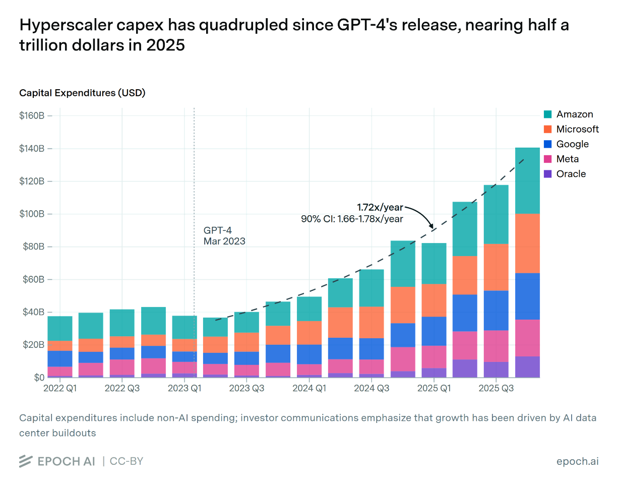
Source: Epoch AI — hyperscaler capex
Extrapolating these trends naively would lead to the following compute forecast:
The method is H100e added = capex × cost-efficiency, both extrapolated naively from the trends above (capex ~1.72×/yr; H100e per $ ~1.4×/yr). 2024/25 are actual Epoch data (AI Chip Sales: 5.09M H100e added on $260B spending in 2024, 13.6M from $448B in 2025).
The rest of this section will attempt to improve the forecast from this naive baseline.
Improving the capex forecast
Through 2025 the buildout was paid for almost entirely out of big-tech's operating cashflow. However, if this trend continues capital expenditures are on track to overtake operating cash flow of hyperscalers around Q3 2026.
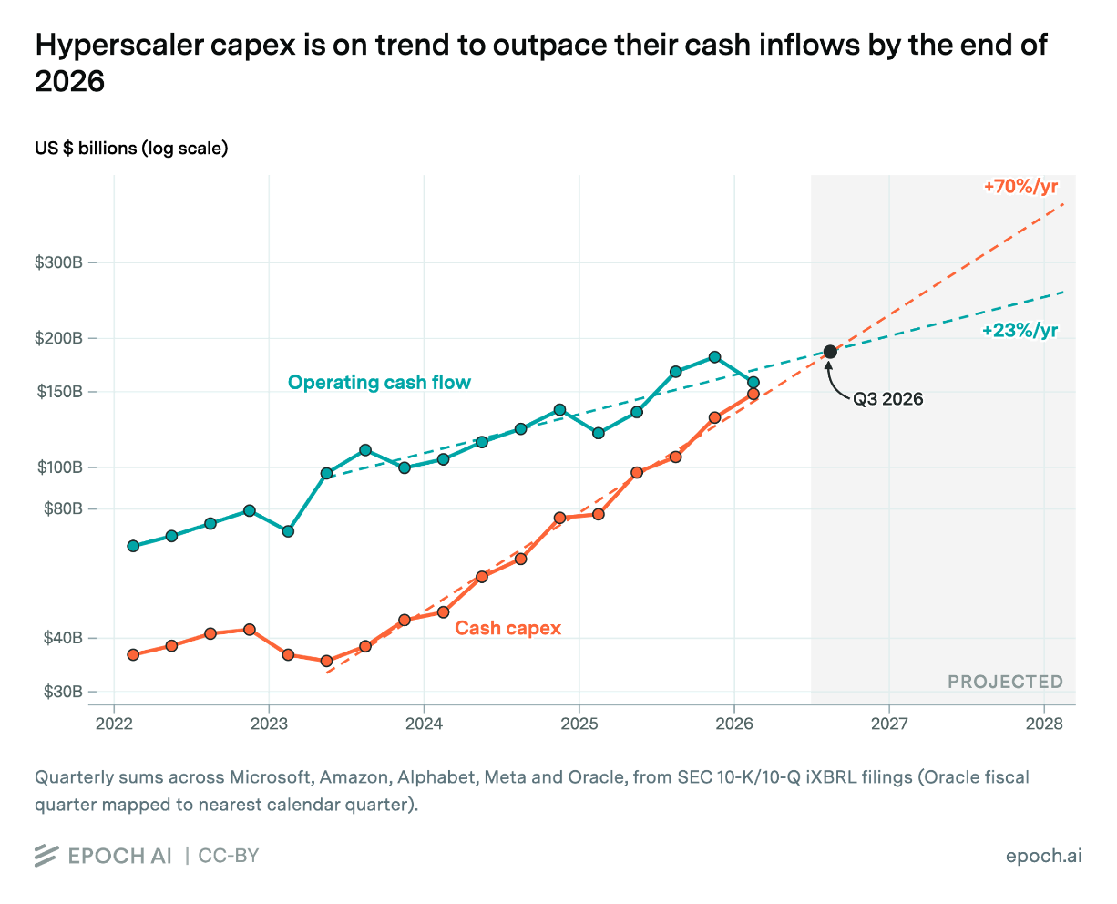
To make a forecast that takes this into account, we split capex projections into three sources: existing-trend hyperscaler cash flow, AI cash flow (additional compute spend from AI company revenues, approximated as 80% of frontier AI company revenue forecasts), and debt & equity raises (which we are already starting to see grow in 2025/2026).
Our projections are as follows:
Existing-trend hyperscaler cash flow to continue growing at ~20%/yr (Epoch's ~$478B → $603B, with frontier AI company revenue stripped out) and deploy a rising share of it into the buildout, an invested fraction climbing ~75 → 85% as capex consumes more of cash flow.
AI cash flow to follow a total ARR (across frontier AI companies) of $30B (start-2026) → $180B → $500B → $1T (start-2029), with 80% of the recognized revenue counted as additional compute spend.
Debt & equity raises are hand forecasted (low effort) as a declining multiple of AI revenue: 3x (2025), 2.8x (2026), 1.8x (2027), 1.6x (2028). This is highly uncertain: on the one hand AI revenue growth motivates leverage, but as the total debt raise grows the interest rate will likely get higher. Note also that leverage at these levels implicitly conditions on the scenario's fast AI progress continuing (lenders keep believing in the revenue growth); like the revenue path itself, it is an input consistent with this scenario rather than an unconditional forecast.
With 2024-25 pinned to Epoch's Broad CapEx ($260B / $448B), this carries total AI capex to ~$2.4T in 2028, with debt reaching ~$900B (38% of the 2028 buildout). (We use hyperscaler Broad CapEx as the proxy for total AI capex: hyperscalers are ~60-90% of global AI spend, and ~60-90% of their capex is AI, and we assume the two gaps roughly cancel.) This is 7% higher than the naive baseline's (extrapolating the ~1.72x/yr trend) 2028 capex of $2.28T! This is because our bullish AI revenue forecast (and the debt raises we think its fast growth will motivate) actually pulls the trend slightly upwards.
Total AI capex = Epoch’s hyperscaler Broad CapEx directly ($260B / $448B for 2024/25). We think hyperscalers are ~60–90% of global spend and ~60–90% of their capex is AI, so we assume the two roughly cancel as a simplifying assumption. Hyperscaler cash flow (existing trend) excludes frontier-AI revenue (to avoid double-counting) and we project it to grow ~20%/yr, with a rising fraction invested (~75→85%). AI cash flow is the additional compute spend from AI company revenues, approximated as 80% of frontier AI company revenue forecasts. Debt & equity raises we hand-pick as a declining multiple of AI revenue (3× / 2.8× / 1.8× / 1.6× for 2025–28), reaching ~$923B by 2028. This leads to ~$2.4T capex in 2028.
AI revenue and debt forecasts
Our AI revenue forecast follows a total frontier AI company ARR (annualized revenue run-rate) path of $30B → $180B → $500B → $1T (year-boundaries 2026.0 through 2029.0). Note that AI revenue is the flow recognized over the year, not the ARR run-rate, so this converts to annual recognized revenue of 2025: $15B / 2026: $84B / 2027: $313B / 2028: $721B. We count 80% of this as additional compute spend (the "AI cash flow" stream above) giving: $12 / $67 / $251 / $577B. Our total frontier AI company ARR projection is done manually and is highly uncertain. Broadly speaking we expect Anthropic's recent ~10x/yr ARR trend to slow down as they become the leading AI company in terms of revenue, and for the overall total AI company revenue trend to return to roughly 3x/yr, and slightly lower as companies manage to maintain roughly flat revenue / inference-compute ($/FLOP) while their inference-compute grows around 2x/yr in the later years. This is somewhat circular with the compute numbers, but is our current (highly uncertain) expectation.
What's a reasonable debt-raising rate given this revenue trend? For starters, the five hyperscalers issued ~$121B of bonds in 2025 (vs a ~$28B/yr 2020-24 norm), with BofA/JPMorgan projecting ~$175-300B in 2026; debt-funded neoclouds like CoreWeave carry ~4x revenue in debt ($21B on ~$5B revenue); and this Morgan Stanley podcast sees ~$1.15T of the ~$2.9T 2025-28 buildout as debt-financed. Total US investment-grade issuance is ~$1.5T/yr. The SpaceX IPO also shows the potential for large equity raises that might be followed with similar/larger ones by OpenAI and Anthropic. We use these anchors to manually set debt as an ad-hoc multiple of total AI revenue, 3x (2025) → 2.8x (2026) → 1.8x (2027) → 1.6x (2028), giving debt-financed AI capex of ~$36B / $188B / $452B / $923B over 2025-2028. That sums to ~$1.6T of debt-financed spending out of the ~$5.1T total buildout (2025-2028; ~31% debt-financed), roughly 39% above Morgan Stanley's ~$1.15T of debt, and ~75% above their ~$2.9T total, respectively, though notably Morgan Stanley's numbers ignore equity-raises.
Improving the cost efficiency forecast (supply-side)
The capex forecast is a demand-side forecast, while for cost-efficiency it makes sense to look at supply side. In particular, this section will focus on lithography (primarily EUV) capacity as the primary expected bottleneck on how many H100e can be produced.
EUV is needed for leading-edge logic, and the leading HBM DRAM nodes now use it too (DRAM was manufactured entirely without EUV until recently, e.g., Micron only adopted it in 2025, so this is a cost-optimality choice rather than a strict requirement; avoiding EUV just shifts the same demand onto the shared DUV pool). EUV is extremely hard to scale on short notice given the complexity of the machines and extensive supply chain dependencies, so we expect it to be the most important and informative bottleneck. Because of the time-inelasticity (how hard it is to quickly scale production in response to price signal), the EUV fleet is also relatively easy to forecast.
| Year | EUV fleet (start of year) | EUV added / yr | fleet passes / yr | AI logic wafers / yr | AI HBM wafers / yr | AI EUV passes / yr | AI share of fleet |
|---|---|---|---|---|---|---|---|
| 2024 | 220 | +44 | 87M | 0.2M | 1.1M | 7M | 7% |
| 2025 | 264 | +48 | 104M | 0.4M | 2.5M | 15M | 15% |
| 2026 | 312 | +65 | 124M | 0.7M | 4.6M | 34M | 27% |
| 2027 | 377 | +80 | 150M | 1.0M | 8.0M | 68M | 45% |
| 2028 | 457 | +100 | 183M | 1.6M | 13M | 118M | 65% |
| 2029 (no Plan A) | 557 | +125 | 223M | 2.1M | 17M | 172M | 77% |
EUV fleet over time and AI's usage share. The fleet starts at 220 operating tools in 2024 (we estimate ASML had ~127 EUV tools in use at end-2021, then shipped 54/42 in 2022/23, per ASML's annual reports; the full build-up with sources is in the details box below) and grows with its accelerating shipments. The EUV added column is ASML's shipments during the year (ASML guides "60+" for 2026 and ~80 for 2027). Fleet passes/yr is the during-year average fleet x ~360k passes/tool. AI's draw sums its logic wafers (x ~12-24 EUV layers per logic wafer, N4→N2) and its HBM-DRAM wafers (x ~4-7 EUV layers per HBM wafer, accounting for stacking and packaging yields). AI's share climbs ~15% (2025) to ~77% (2029, no Plan A).
How EUV scanners make a H100e
AI's claim on the fleet comes from both logic and memory, so we add the two in a single unit: an EUV pass = one EUV exposure of one wafer (a tool images ~360k/yr regardless of what it's printing). Here is the 2025 build-up.
1. Fleet → passes. Each scanner runs only ~40-50 wph-equivalent in practice, versus a ~160 wafers-per-hour nameplate: real patterns need longer exposures than the spec assumes (higher dose, limited by the light source's power), tools are only up ~75-82% of the time, and time is lost stepping between exposure fields (reticle overhead). Netting these out gives ~360,000 effective passes/tool/yr (the naive 160 wph x 8,760 h ≈ 1.1-1.4M is 3-4x too high). Two back-calculations agree: Frederick Chen (<50 wph effective) and SemiAnalysis (~1,500 wafers/mo x ~20 exposures). Starting from ~220 operating tools at the start of 2024 (ASML had ~127 EUV in use at end-2021, then shipped ~54 and ~42 in 2022-23; TSMC alone runs ~56% of capacity) the fleet does ~100M passes/yr in 2025, growing to ~220M by 2029 as ASML's EUV shipments accelerate (~48 in 2025 toward ~120/yr by 2029).
2. AI's logic draw. AI accelerators take ~0.4M leading-edge wafers in 2025, roughly ~12% of TSMC's ~3M ≤5nm wafers (Epoch's direct estimate; Blackwell on N4, Nvidia only now ramping into N3). At N4's ~14 EUV layers that is ~5M passes. (An ~800mm² die yields ~42 good dies/wafer at ~70% yield, per Cerebras; at ~28-36 H100e/wafer today → ~120 by 2029 as FP4 + the N4→N3→N2 shrink + Rubin's high H100e/chip compound, the all-logic ceiling is ~200M → ~1.2B H100e/yr. The shrink is not free EUV-wise: the model charges a growing pass count per logic wafer, ~12 in 2024 rising to ~24 by 2029, as more layers move onto EUV.)
3. AI's memory draw (the larger half). Essentially all HBM goes to AI, and HBM uses a lot of wafers per GB. Reported 2025 HBM TSV/back-end capacity is ~400k wafers/month (SK Hynix ~170k + Samsung ~165k + Micron ~60k, TrendForce), but that's a capacity ceiling, not utilized starts. Netting yields, AI's actual draw is ~2.5M HBM core-wafers/yr: a 24Gb-die DRAM wafer holds ~1,400 GB gross, and after ~57% core+stacking (KGSD/TSV) yield and ~88% CoWoS-assembly yield only ~700 net GB ship per started wafer, while the 2025 fleet needs ~1.8B GB of HBM (bottom-up: ~11.7M accelerators x ~150 GB, cross-checking the ~$35B / ~2B-GB industry total). The leading HBM nodes use real EUV (SK Hynix 1b ~4 layers, 1c ~6), so at ~4 layers that is ~10M passes, roughly two thirds of AI's EUV draw. (Per GB, HBM burns ~3x a DDR5 wafer.)
4. AI's fleet share. Logic (~5M) + HBM (~10M) = ~15M passes / ~104M fleet ≈ 15% in 2025. Rising HBM volume and EUV-layer count, plus AI's migration onto EUV-heavy N3/N2 logic, carry it to ~64% by 2028 and ~77% by 2029, with AI approaching saturation of the EUV fleet around 2029-30. This draw feeds back into the cost surcharge (more EUV use means a higher surcharge and fewer H100e per dollar), so it is solved self-consistently, and it is what trims the late buildout (2028 additions ~155M vs a naive ~190M).
5. Why passes and not wafer counts. AI's wafers are a mix: an HBM wafer takes only ~4 EUV passes while a leading-edge logic wafer takes ~14-22, so counting wafers treats very different claims on the fleet as equal. Since AI's wafer mix is HBM-heavy, a wafer count overstates its early share (it would put 2025 well above the ~15% the pass count gives). The two measures converge by 2029 for a simple reason: by then AI is the majority user of both the logic and the HBM wafer pools, so the mix difference stops mattering and either way of counting lands around ~80%.
AI's share of the EUV fleet grows from ~7% in 2024 toward ~64% by 2028 (and ~77% by 2029, near saturation). We expect this to translate to higher prices as it requires outbidding other uses of the fleet (e.g., phones, PCs, etc.). To model this, we implement a hand-chosen cost surcharge curve that depends on the fleet usage (highly uncertain ad-hoc choice).
Our forecast for % of global EUV time (passes) used by AI, including both logic and memory wafers (and accounting for yields). It runs ~7% in 2024 toward ~65% by 2028 (~77% by 2029), so AI hits the EUV wall around 2029-30. The cost surcharge (curve tab), surcharge = A·u^K (default A = 100%, K = 2.5), is keyed to this derived path and feeds back into the compute forecast (more draw → higher surcharge → fewer H100e), solved to a fixed point so it climbs to ~33% by 2028 and throttles the late buildout. The K and A sliders tune how hard it bites for users to play with. The parameters are hand chosen and extremely uncertain.
Applying this surcharge to the naive price-performance trend gives an updated compute cost-efficiency trend that averages ~1.25x/yr from 2025-2028 (and slows to just ~1.1x/yr by 2028 as the surcharge bites) instead of the historical ~1.4x/yr.
Cost per H100e decomposes as $ per wafer ÷ H100e per wafer.
Where the wafer numbers come from
The cost figure is an identity, $/H100e = (all-in $/wafer) / (H100e per wafer), and we have decent estimates of two of the three quantities, so we back out wafers per $B (the inverse of all-in $/wafer) as the residual and then check whether the wafer cost it implies is sensible.
$/H100e (known). 2024/25 are observed (annual capex / H100e added: ~$51K, ~$33K). For 2026-28 we take the ~1.4x/yr price-performance trend and penalize it by the EUV surcharge, giving ~$23K / ~$18K / ~$16K.
H100e per wafer (known, ~28 → ~98). An ~800mm² reticle-limit die yields ~64-72 gross dies per 300mm wafer, ~42 good at ~70% yield; netting downstream losses (packaging yield) leaves ~28 sellable H100e per wafer in 2024. This climbs ~1.4x/yr to ~98 by 2028 (~120 by 2029) from FP4/precision (EUV-free), the N4→N3→N2 shrink (paid in extra EUV layers), and Rubin's high H100e/chip, all reasonably well grounded in die-size, node, and precision estimates. (2025 check: ~13.6M H100e on ~0.38M AI leading-edge wafers ≈ ~36 H100e/wafer.)
Wafers per $B (the residual). Multiplying the two backs out the implied all-in $/wafer: ~$1.43M (2024) → ~$1.18M (2025) → ~$1.20M → ~$1.36M → ~$1.56M (2028), i.e. wafers/$B ~700 → ~845 → ~640. The 2025 dip comes directly from the observed data: 2024 was early and supply-constrained, and 2025 hit Blackwell volume, so all-in cost per leading-edge wafer fell. From 2026 the implied $/wafer rises, which is what we'd expect: TSMC ASP +5-10%/yr (N2 ~$30K, +10-20% over N3), CoWoS +15-20%/yr, datacenter $/MW rising, plus the EUV surcharge. The level also checks against a bottom-up per-wafer build-up: foundry ~$25-30K, HBM for the wafer's ~28 dies ~$50-70K, CoWoS ~$10-15K, and a ~4-5x chip-designer markup giving ~$400-500K of accelerator value per wafer (roughly $15K per accelerator); the remaining ~$0.7-1.1M per wafer (~$25-40K per accelerator) is the non-chip buildout: datacenters, power, land, networking. So the residual looks reasonable: wafer costs are a mild headwind after 2025, and the whole ~$51K to ~$16K decline in $/H100e comes from compute density improvements.
Multiplying this cost-efficiency baseline (incl. the scarcity surcharge) by the capex topline gives the annual H100e added (~155M in 2028), and an installed stock of ~280M by end-2028. We also adjust very slightly downwards for chip survival rates. China's domestically manufactured compute (§1.3) does not draw on this EUV supply chain, so we forecast it separately and add it onto this total, bringing the world AI stock to ~287M.
H100e added is annual capex × cost-efficiency (anchored to the 2024/25 actuals 5.09M, 13.6M, then forecast); installed stock is shown at the end of each year. The black bars are the EUV-constrained §1.1 buildout (~155M added in 2028, ~280M installed by end-2028); the red caps add China’s off-EUV domestic manufacturing (§1.3), for a ~289M world total. Toggle ‘effective’ to rescale by the §1.2 usefulness factor.
Resource intensity: from raw H100e to effective compute
Even for the AI fleet, effective and raw H100e drift apart. The memory wall drags effectiveness below 1 (TPP, boosted by FP4, outgrows HBM bandwidth and capacity), while the growing coherent NVLink world (HGX-8 → NVL72 → NVL144 → NVL576) pushes it back up. The two roughly cancel: there is a mild premium in 2024 (~1.16, when the fleet is memory-rich) that fades toward ~1 by 2029 as the memory wall and larger training runs start to matter more. It is the same usefulness model as §1.2.3 (full derivation in the appendix); the deployment-weighted fleet inputs that drive it (scale-up world in H100e = coherent chips x H100e/chip):
| AI fleet (deployment-weighted) | 2024 | 2026 | 2028 |
|---|---|---|---|
| HBM bandwidth per H100e (GB/s) | 4,080 | 3,330 | 3,610 |
| HBM capacity per H100e (GB) | 110 | 91 | 85 |
| scale-up world (H100e) | 184 | 436 | 929 |
| H100e per chip | 1.15 | 2.58 | 5.34 |
| effective H100e per raw | 1.16 | 1.06 | 1.04 |
1.2 All compute
§1.1 forecast AI-relevant compute. Now we extend to all compute in the world. We split all compute into six device categories:
| Category | Examples | AI-relevant |
|---|---|---|
| AI | datacenter AI accelerators (H100, B200, MI300) | yes |
| Non-AI servers | datacenter CPUs and non-AI accelerators | no |
| PCs | laptops and desktops | no |
| Phones | smartphones | no |
| Gaming | gaming GPUs | no |
| Other | microcontrollers, automotive, edge | no |
Our method works by looking at two quantities. The device side is the compute we get from counting the units shipped and the average compute carried on each device. The lithography side is the compute the world can make, from counting the wafers the fabs can produce and the compute each wafer turns into.
device side H100e = units H100e per unit
lithography side H100e = wafers H100e per wafer
The compute per wafer is the quantity we are least sure of, so it is what we attempt to pin down from history (where we can get good estimates of all the other values).
1.2.1 Calibration (2015 to 2024)
Across 2015 to 2024 we look at device demand (units shipped and compute per unit) and lithography supply (wafers shipped), and use this to back out an estimate of compute per wafer that we can then use to forecast future compute by category based on wafer allocation and wafer supply forecasts (which are easier to do than device demand forecasts, because the supply side can be forecasted with the relatively predictable lithography ceiling).
Device side
| Shipments (M units/yr) | 2015 | 2018 | 2020 | 2022 | 2024 |
|---|---|---|---|---|---|
| phones | 1K | 1K | 1K | 1K | 1K |
| pcs | 276 | 259 | 304 | 292 | 263 |
| gaming | 44 | 50 | 40 | 38 | 36 |
| ai | 0.1 | 0.3 | 0.6 | 2.0 | 7.5 |
| non-AI servers | 8.0 | 11 | 13 | 14 | 13 |
| other | 12K | 20K | 24K | 28K | 30K |
Shipment sources
- phones: 1.43B (2015) → 1.24B (2024). Peak 1.47B (2016); pandemic trough 1.21B (2022). Source: IDC Worldwide Quarterly Mobile Phone Tracker / Omdia / Counterpoint.
- pcs: 276M (2015) → 263M (2024). COVID peak ~349M (2021), trough ~260M (2023). IDC runs ~30M above Gartner in 2020 to 2021 because IDC counts Chromebooks; we use the IDC basis. Source: Gartner / IDC PCD Tracker.
- gaming: discrete desktop add-in-board GPUs only (not iGPUs, not datacenter). 44M (2015) → ~35M (2024). Source: Jon Peddie Research AIB Report.
- ai: the whole AI datacenter; unit count = accelerators. TechInsights counted 3.76M NVIDIA datacenter GPUs in 2023 (98% share); 2024 is ~7.5M all-vendor (NVIDIA ~4M + Google TPU ~2.5M + AWS Trainium ~1.2M + AMD MI300 ~0.4M). Source: TechInsights via DCD; Epoch AI; Omdia/Morgan Stanley.
- other: just the advanced-node digital chips (networking ASICs, basebands, auto/IoT logic). The full MCU plus analog universe is far larger (~25 to 35B MCUs/yr alone), but most is trailing-node / 200mm capacity outside the 300mm lithography pool this model tracks.
| TPP per unit | 2015 | 2018 | 2020 | 2022 | 2024 |
|---|---|---|---|---|---|
| phones | 0.5 | 5.0 | 25 | 60 | 100 |
| pcs | 8.0 | 20 | 38 | 62 | 100 |
| gaming | 15 | 250 | 550 | 1K | 2K |
| ai | 350 | 1K | 2K | 5K | 10K |
| non-AI servers | 30 | 75 | 150 | 320 | 500 |
| other | 0.1 | 0.3 | 0.5 | 0.7 | 0.9 |
TPP-per-unit sources
TPP = (peak dense TOPS at a precision) × (bit-length of that precision), maximized over precisions: the US BIS export-control metric (ECCN 3A090). Anchors that fix the scale: V100 ≈ 2,000, A100 = 4,992, H100 ≈ 15,800, RTX 4090 = 5,285 (just over the 4,800 control line), B200 ≈ 36,000. All figures are sales-weighted averages, since the flagship is a tiny share of units. Sources: Federal Register 88 FR 73458, CSET explainer, Princeton ISCA 2025.
- phones: NPU INT8 TOPS × 8. Apple A11 = 0.6 TOPS (2017) → A17 Pro = 35 TOPS (2023); Snapdragon 8 Gen 3 = 45 TOPS (2024). Near-zero before 2017. Sales-weighted ≈ 100 TPP in 2024. Source: Apple Neural Engine TOPS table.
- pcs: most PCs have no NPU (only ~17% of 2024 units were “AI PCs”). Sales-weighted ≈ 100 TPP in 2024. Source: Canalys AI-PC share.
- gaming: dense INT8 TOPS × 8: RTX 3060 = 815, RTX 4060 = 968 (4060 Ti = 1,412), RTX 4090 = 5,285. The sales mix is mostly xx60-class (Steam survey), so the sales-weighted average is ~1,500 TPP in 2024, not the 4090’s 5,285. Source: Steam Hardware Survey.
- ai: sales-weighted across all vendors (H100/H200 = 15,800, A100 ≈ 5,000, TPU/Trainium lower), 2024 ≈ 9,500 TPP, below the NVIDIA flagship. With ~7.5M units that gives ~4.5M H100e in 2024, the bottom-up value that meets the Plan A forecast at the 2025 seam. Source: NVIDIA/Google/AWS datasheets; TrendForce mix.
- other: ~30B chips/yr, mostly MCUs/analog with ~0 AI throughput; only a thin automotive/ADAS + edge-NPU tail carries any, so the unit-weighted average is just ~1.5 TPP by 2024.
Lithography side
| wafers (M/yr) | 2015 | 2018 | 2020 | 2022 | 2024 |
|---|---|---|---|---|---|
| phones | 1.8 | 1.9 | 1.9 | 1.9 | 2.1 |
| pcs | 0.7 | 0.7 | 0.9 | 0.9 | 0.9 |
| gaming | 0.2 | 0.3 | 0.2 | 0.3 | 0.3 |
| ai | 0.0 | 0.0 | 0.0 | 0.0 | 0.3 |
| non-AI servers | 0.1 | 0.2 | 0.3 | 0.3 | 0.3 |
| other | 5.5 | 9.7 | 12 | 15 | 17 |
| device demand (total) | 8.3 | 13 | 15 | 18 | 20 |
Wafer shipment sources
- Each category’s wafers = its logic wafers (units × dies-per-device ÷ good-dies-per-wafer) plus the memory wafers (HBM, DRAM, NAND) that ship with it. Units are the shipments table above. Memory wafers follow from each device’s memory content and current per-wafer GB on DRAM/NAND/HBM nodes.
- Good dies per 300mm wafer (yield-net): phones ~600 (~100 to 120 mm²), PCs ~300 (~200 mm²), gaming ~130 (~400 mm²), AI ~42 (~800 mm² reticle-limit die at ~70% yield), “other” ~1,800 (~30 mm²). Sources: AnySilicon; reticle/die-size disclosures (TSMC, NVIDIA, WikiChip).
- Dies per finished device: non-AI ≈ 1 (one SoC/CPU/GPU per device). AI ramps 1 (H100) → ~1.5 (2024, dual-die B200) → ~8 to 11 by 2030 (Rubin-class chiplets). Sources: NVIDIA roadmap; SemiAnalysis.
- Die-area is already net of yield, so no separate yield factor is applied.
The lithography utilization by category is shown below. We treat every category as a package with its logic and associated memory (HBM, DRAM, NAND).
EUV exposure-passes drawn per year (the absolute view the share hides). Volume EUV begins ~2019; it’s ~all phones/PCs early, AI invisible until ~2022.
Sanity check with independent compute per wafer estimates
Compute per wafer is just (good dies per wafer) x (TPP per die) / 15,800, both estimated from device specs independently of how full the fabs run:
Good dies per 300mm wafer (yield-net, from die areas; sources in the wafer box above): AI ~42 (an ~800 mm² reticle-limit die at ~70% yield), gaming ~130 (~400 mm²), PCs ~300 (~200 mm²), phones ~600 (~100 to 120 mm²), commodity 'other' ~1,800 (~30 mm²).
TPP per die = each category's TPP per unit (device side above) / its dies per device. In 2024 AI is ~9,500 / ~1.5 ≈ 6,300 TPP/die, gaming ~1,500, phones and PCs ~100, 'other' ~1.5.
So AI's big, high-TPP dies make it densest per wafer and commodity 'other' (tiny, near-zero-TPP dies) the lowest, which is exactly what dividing each category's compute by its wafers gives:
| implied H100e / wafer | 2015 | 2018 | 2020 | 2022 | 2024 |
|---|---|---|---|---|---|
| phones | 0.03 | 0.23 | 1.1 | 2.4 | 3.8 |
| pcs | 0.20 | 0.46 | 0.83 | 1.3 | 1.9 |
| gaming | 0.19 | 2.8 | 5.6 | 9.2 | 12.3 |
| ai | 1.4 | 5.0 | 7.2 | 14.2 | 16.8 |
| non-AI servers | 0.11 | 0.25 | 0.46 | 0.90 | 1.3 |
| other | 0.01 | 0.04 | 0.06 | 0.09 | 0.10 |
As a further check, the wafer demand these rates imply, set against our estimated lithography pool (broad global logic-wafer output, ~30M wafers in 2024, a scale consistent with SEMI's 300mm capacity), is ~62% to ~69% of the pool across the decade: a plausible, stable share that never runs past the pool. The pool level is itself calibrated to land in that range, so this says the die-size, compute, and capacity estimates are mutually consistent rather than independently validating any one of them.
The resulting H100e added each year by category is shown below in both raw and effective H100e:
Raw H100e added per year by category.
1.2.2 Forecast (2025 to 2028)
We take AI's compute forecast from §1.1 and ration the leftover lithography capacity to the other compute categories. AI first claims its lithography usage and then each non-AI category keeps its frozen-2024 share of the wafers that remain. That gives the projection:
| Flow (H100e/yr) | 2025 | 2026 | 2027 | 2028 |
|---|---|---|---|---|
| phones | 12.0M (33%) | 16.6M (25%) | 21.5M (18%) | 31.0M (14%) |
| pcs | 2.8M (7.7%) | 4.1M (6.2%) | 5.5M (4.5%) | 8.8M (4.0%) |
| gaming | 5.2M (14%) | 7.2M (11%) | 9.4M (7.8%) | 14.2M (6.5%) |
| ai | 14.2M (39%) | 35.7M (54%) | 80.6M (67%) | 159.7M (73%) |
| non-AI servers | 558K (1.5%) | 725K (1.1%) | 901K (0.7%) | 1.2M (0.5%) |
| other | 2.0M (5.4%) | 2.3M (3.4%) | 2.6M (2.2%) | 3.2M (1.5%) |
| total | 36.7M | 66.6M | 120.5M | 218.1M |
AI is from §1.1; non-AI gets the leftover logic wafers × rising TPP-per-wafer. Counting logic + HBM, AI reaches ~15% → 65% of EUV fleet capacity by 2028 (with the fleet ~100% utilized overall), but only ~40% of all logic wafers.
AI’s wafer claim, leftover pool, and bill of materials
| wafers/yr | 2025 | 2026 | 2027 | 2028 |
|---|---|---|---|---|
| AI logic wafers | 378K | 664K | 1.0M | 1.6M |
| + AI HBM wafers (advanced DRAM) | 2.5M | 4.6M | 8.0M | 12.8M |
| = AI cutting-edge wafers (logic + HBM) | 2.9M | 5.2M | 9.1M | 14.4M |
| % of EUV fleet capacity (logic + HBM) | 15% | 27% | 45% | 65% |
| % of broad lithography pool (all nodes) | 9.3% | 16% | 27% | 40% |
| allocatable logic pool (× util) | 20.9M | 22.0M | 23.2M | 24.4M |
| leftover for non-AI | 20.6M | 21.4M | 22.1M | 22.8M |
Sources: AI forecast and per-accelerator bill of materials
- AI H100e trajectory. From §1.1’s EUV-constrained solve (capex topline ÷ cost-efficiency ÷ EUV surcharge): installed H100e stock (Jan-1) 8.6M · 22.4M · 57.1M · 135.2M → 289.0M by 2029, with annual production 14.2M · 35.7M · 80.6M · 159.7M. §1.2 takes this AI buildout from §1.1 unchanged and models only the non-AI leftover, so the two sections agree by construction. Source: §1.1 (resting on the Plan A capex topline).
- HBM per accelerator. H100 = 80 GB, H200 = 141, MI300X = 192, B200 = 192; sales-weighted ~130 GB in 2024 → ~600 by 2030. × ~7.5M units ≈ 1 EB HBM in 2024, matching the TrendForce industry figure. Source: NVIDIA/AMD datasheets; TrendForce.
- System DRAM & storage per accelerator. An 8-GPU node carries ~1 to 2 TB host DRAM (~150 to 250 GB/GPU) plus multi-TB local + networked NVMe. We model ~300 GB DRAM and ~2 TB NAND per accelerator in 2024 (growing to ~1 TB / ~6 TB by 2030), sized so HBM stays AI’s heaviest wafer draw, not the commodity memory. Source: NVIDIA DGX/HGX H100 specs; hyperscaler reference designs.
- Stock vs production convention. AI’s fleet is treated as cumulative (no retirement over this <5-yr window), so each Jan-1 stock is the running sum of production; we take the stock directly rather than running the bottom-up retirement recursion used for the non-AI categories. The production figure drives each year’s wafer claim.
The rest of this section is the supply-side justification behind that table, i.e., what share of the lithography ceiling each category uses.
EUV exposure-passes drawn per year. AI’s draw explodes, taking the fleet toward saturation by 2028.
Share of EUV and DUV passes that go to logic vs. memory
EUV utilization reaches ~100% by 2028 in our naive model, up from only 52% in 2024, as we expect it to become the binding constraint by then. That figure already separately accounts for uptime and realized throughput, both held at 2024 proportions. We don't expect utilization to literally hit 100%, but we're comfortable with the approximation: uptime and realized throughput (as a share of peak theoretical throughput) should improve a bit by 2028, roughly offsetting the gap.
| EUV pass pool (M/yr) | 2024 | 2028 |
|---|---|---|
| passes demanded | 45.3M | 182.5M |
| pass capacity | 87.1M | 182.5M |
| EUV utilization | 52% | 100% |
| immersion (DUV) utilization | 20% | 25% |
Utilization = passes demanded ÷ pass capacity. EUV and immersion are both on the effective (uptime- and throughput-adjusted) basis, so the two utilizations compare directly.
Node structure: passes per wafer and node mix
| node | EUV/wf | 193i/wf | wafers 2024 | wafers 2028 |
|---|---|---|---|---|
| logic tiers | ||||
| LEADING | 12→22 | 30 | 2.0M | 3.2M |
| DUVADV | 2 | 33 | 2.0M | 5.2M |
| MATURE | n/a | 6 | 16.4M | 16.0M |
| memory tiers | ||||
| DRAMadv | 4 | 12 | 4.2M | 20.7M |
| DRAMmat | n/a | 8 | 5.8M | 7.6M |
| NAND | n/a | 4 | 40.2M | 45.0M |
Three tiers (LEADING = ≤N3/N5/N2, EUV; DUVADV = N7/N16; MATURE = 28nm/legacy). Leading EUV passes/wafer climb 12→22 as the mix shifts N5→N3→N2. Red = EUV-drawing. This grid is a utilization diagnostic; it does not feed the compute or stock math.
Node mix (2024 wafer-area share by category)
| category | LEADING | DUVADV | MATURE |
|---|---|---|---|
| phones | 53% | 27% | 20% |
| pcs | 42% | 40% | 18% |
| gaming | 55% | 45% | n/a |
| ai | 95% | 5.0% | n/a |
| non-AI servers | 50% | 42% | 8.0% |
| other | n/a | 5.0% | 95% |
AI is ~all leading-edge; phones/PCs/gaming span leading to mature; “other” (MCUs) is ~all mature. The broad logic pool (29.5M wafers in 2024) feeds the non-AI allocation.
Per-device memory and wafer cost
Memory wafers = device count × per-device GB ÷ GB-per-wafer. HBM needs ~3× the wafer area per usable GB (8 to 12-hi stacks, TSVs, a base logic die) and goes almost entirely to AI, so an AI accelerator’s memory outweighs its logic on wafers.
| per device (2024 → 2028) | HBM | DRAM | NAND |
|---|---|---|---|
| phones | n/a | 8 → 13 GB | 200 → 333 GB |
| pcs | n/a | 16 → 27 GB | 700 → 1033 GB |
| gaming | n/a | 14 → 21 GB | n/a |
| ai | 130 → 400 GB | 300 → 767 GB | 2000 → 4667 GB |
| non-AI servers | n/a | 512 → 683 GB | 26000 → 36667 GB |
| other | n/a | 0.05 → 0.05 GB | 2 → 3 GB |
- GB per wafer (2024): DRAM ~2,800, NAND ~21,000, HBM ~900; all grow ~1.7× by 2030. HBM is ~11% of DRAM wafers in 2024 (TrendForce: ~14%). Sources: SEMI; TechInsights; TrendForce.
- The non-AI server row carries the datacenter storage tier (SSD arrays, networked NVMe), so its NAND is large (~26 TB/server-equivalent); this folds in bulk storage a strict per-device count misses, landing world NAND ≈ 845 EB in 2024 (~44M wafers), in line with Trendfocus. Sources: TrendForce; Trendfocus; IDC / Omdia.
Litho supply sources: EUV layers/node, fleet, throughput, node mix
- EUV layers per node: N5/N4 ≈ 13 to 14, N3E ≈ 19, N3B ≈ 25 (double-patterned), N2 ≈ 23 to 25. A double-patterned layer needs two exposures, so passes ≥ layers; we model the leading tier climbing 12→24 (2024→2029). Sources: SemiAnalysis; WikiChip; TSMC.
- Memory EUV: advanced DRAM (1α/1β/1γ) uses ~1 to 6 EUV layers, ramping; 3D NAND uses none. We model advanced DRAM at ~4 EUV passes/wafer, mature DRAM and NAND at 0. Sources: SK Hynix / Samsung / Micron disclosures; TechInsights.
- EUV fleet: ~220 systems by 2024, ~457 by 2028 on ASML guidance. Throughput: ~360k effective exposures/tool-year (below the ~160 wph spec). Source: ASML.
- Immersion fleet: ~1,330 (2024) → ~1,800 (2028); abundant, so 193i never binds. Throughput: ~950k effective passes/tool-year (about half the ~1.8M nameplate run-rate, de-rated on the same uptime/throughput basis as EUV). Node mix is wafer-area share: Counterpoint ~43% of 2024 phone-SoC units on ≤5nm → ~53% of wafer area. Sources: ASML / SEMI; Counterpoint; TSMC.
1.2.3 Results
Accumulating production net of retirement gives the installed stock by category. Rescaling raw H100e to effective H100e (raw x , the resource-adjusted AI workload usefulness model derived in the appendix).
Effective H100e rescales each category’s raw compute by a usefulness factor U, derived in the appendix.
| usefulness U | 2024 | 2026 | 2028 | 2029 |
|---|---|---|---|---|
| phones | 0.21 | 0.11 | 0.07 | 0.05 |
| pcs | 0.35 | 0.08 | 0.04 | 0.03 |
| gaming | 0.04 | 0.05 | 0.06 | 0.04 |
| ai | 1.16 | 1.06 | 1.04 | 1.02 |
| non-AI servers | 1.38 | 1.40 | 1.41 | 1.40 |
| other | 0.53 | 0.43 | 0.34 | 0.30 |
Per-chip inputs and the unclamped model output
The per-chip resource inputs that drive U, by category (2024). Only AI accelerators pair real compute with HBM-class bandwidth and a large NVLink coherent domain; every other category is effectively a single chip (scale-up world = 1). Non-AI servers are memory-rich but compute-light; consumer chips are bandwidth-poor and don’t cluster; “other” (MCU / edge) is tiny on every axis.
| per chip (2024) | H100e/chip | mem BW (TB/s) | mem (GB) | scale-up world |
|---|---|---|---|---|
| phones | 4.0e-3 | 0.032 | 7 | 1 |
| pcs | 6.6e-3 | 0.085 | 12 | 1 |
| gaming | 0.097 | 0.41 | 11 | 1 |
| ai | 1.15 | 4.7 | 126 | 160 chips |
| non-AI servers | 0.030 | 0.70 | 512 | 1 |
| other | 5.7e-5 | 0.006 | 0.1 | 1 |
Over the forecast, H100e/chip roughly doubles every ~1.5 years while memory bandwidth and capacity per H100e fall (the memory wall) and AI’s NVLink world grows (NVL72 â NVL576); the §1.1 resource-intensity box tracks the AI fleet’s trajectory in full.
Raw U, before the non-AI ≤ 1 cap
| category (raw U) | 2024 | 2026 | 2028 | 2029 |
|---|---|---|---|---|
| phones | 0.21 | 0.11 | 0.07 | 0.05 |
| pcs | 0.35 | 0.08 | 0.04 | 0.03 |
| gaming | 0.04 | 0.05 | 0.06 | 0.04 |
| ai | 1.16 | 1.06 | 1.04 | 1.02 |
| non-AI servers | 1.38 | 1.40 | 1.41 | 1.40 |
| other | 0.53 | 0.43 | 0.34 | 0.30 |
Servers and “other” (MCU/edge) score > 1 because for a tiny-compute chip every per-FLOP ratio looks abundant, so the networking penalty all but vanishes and it floats to the compute ceiling. For non-AI servers this is plausible (genuinely memory-rich machines) and they are tiny in raw H100e (~1–2%), so we keep their raw U. For MCU/edge “other” it is an artifact, so we clamp it to ≤1; note “other” is a large raw share (~8–23%), so even the clamp at 1 likely overstates its AI usefulness.
Installed H100e on Jan 1 of each year by deployment quadrant; toggle stock↔flow, raw↔effective, and level↔share.
Cluster vs. single-device split. We also categorize compute into clusters and single-devices. Non-AI servers are treated as non-AI relevant clusters; phones, PCs, gaming GPUs and embedded chips are non-AI single-device; and AI relevant compute is almost entirely in accelerators run in datacenters (AI-relevant clusters), but there is a small rising amount of AI-relevant single-device chips that is negligible today and grows later as datacenter-class GPUs reach desktop form factors (e.g., NVIDIA's DGX Station).
| effective H100e stock (Jan 1) | 2020 | 2024 | 2026 | 2028 | 2029 |
|---|---|---|---|---|---|
| AI-relevant · cluster (AI datacenters) | 101K (4.1%) | 3.6M (26%) | 23.7M (67%) | 140.8M (90%) | 295.2M (94%) |
| AI-relevant · single-device (specialty consumer) | 0 | 0 | 0 | 218K (0.1%) | 938K (0.3%) |
| non-AI · cluster (non-AI servers) | 294K (12%) | 1.4M (10%) | 2.6M (7.5%) | 4.7M (3.0%) | 6.1M (1.9%) |
| non-AI · single-device (consumer) | 2.1M (84%) | 8.7M (63%) | 9.1M (26%) | 11.5M (7.3%) | 12.6M (4.0%) |
How we forecast AI-relevant single-device compute (specialty consumer)
These are standalone AI workstations: a capable GPU (≥1 TB/s bandwidth, ≥32 GB, ≥4,000 TPP) paired with a 100 Gb/s NIC, which clears all four AI-relevant floors. They range from workstations on RTX PRO 6000-class GPUs up to NVIDIA’s DGX Station (one GB300, ~2.5 H100e). Cheaper minis like DGX Spark (~0.5 H100e) miss the bandwidth floor, and ordinary gaming PCs lack the 100 Gb/s NIC. At ~$10,000 to ~$100,000 each, they sell in modest volumes. We estimate units sold per year and H100e per unit, then add them up.
| shipping year | units shipped | H100e / unit | H100e added | installed (Jan 1) |
|---|---|---|---|---|
| 2026 | 15K | 2.5 | 38K | 0 |
| 2027 | 60K | 3 | 180K | 38K |
| 2028 | 180K | 4 | 720K | 218K |
| 2029 | 450K | 5 | 2.3M | 938K |
The installed (Jan 1) column is the running stock at the start of each year — exactly the specialty-consumer row in the table above (~938K H100e by 2029.0, about 0.3% of the AI fleet, ~255K units). The category is new, so the unit numbers are rough estimates.
1.3 Regional ownership
This section forecasts world compute ownership by region, for the AI-relevant compute from §1.1. We split ownership three ways: US, China, and the Rest of the World. We think it is most informative to focus on a separate Chinese compute forecast, because China is cut off from the main global supply chain by export controls, making it the hardest region to pin down with a crude percent-of-spending estimate.
What follows is therefore an independent Chinese compute forecast, broken down by the different sources of compute reaching China. We then make a crude estimate of the US versus Rest-of-World split of the global total. China's domestic manufacturing is treated as separate from the world compute total forecast in §1.1, because it does not come from the same (EUV-based) supply chain, so the §1.1 totals add it back on.
1.3.1 Chinese compute forecast
We categorize China's AI compute into four sources: Three come from the global supply chain (already in the §1.1 world total): legal imports (export-compliant chips: e.g., H20s historically, H200 under the current licensing policy), smuggled chips, and loopholes (chip dies smuggled in before packaging, or offshore datacenters Chinese firms own or lease from abroad). The fourth is domestically manufactured chips (SMIC 7nm logic / CXMT HBM / Ascend). China's compute grows ~9x over 2026-2029, but its world share still falls toward ~9% because the global buildout outpaces it.
The 2024-2025 anchors, pinned to observed data:
| Channel | 2024 | 2025 | Basis |
|---|---|---|---|
| Domestic | 0.25M | 0.6M | Ascend on SMIC ≤7nm + Cambricon, drawing a one-time foreign-HBM stockpile (~13M stacks, mostly Samsung ~11.4M ≈ 1.6M 910C) and a ~2.9M-die TSMC "die bank" (SemiAnalysis); ~0.8 raw H100e/910C |
| Legal | 0.2M | 0.15M | ~1M throttled H20s in 2024 (~0.2 H100e each); 2025 nets only ~0.15M: Q1 shipments before the April ban, a partial re-licensing from July, and Beijing discouraging purchases |
| Loopholes | 0.25M | 0.45M | offshore DCs Chinese firms own or rent abroad; the cumulative 2024+2025 total here (~0.7M by end-2025) sits just above the ≥~670K confirmed-rental floor (ByteDance ~520K) |
| Smuggled | 0.16M | 0.48M | grey-market banned parts, anchored to Epoch |
Forecasting 2026-2028
The three global channels are projected as a share of §1.1 world production:
| Global channel | Rule (share of §1.1 world) | 2026 | 2027 | 2028 |
|---|---|---|---|---|
| Smuggled | ~3.5% → 2% with more enforcement | 1.26M | 2.12M | 2.99M |
| Loopholes | ~2% (~1.5% confirmed-rental floor + other sources) | 0.7M | 1.6M | 3.15M |
| Legal | ~1% | 0.35M | 0.8M | 1.6M |
The legal channel could plausibly run 2-3x higher than this ~1% rule: the current licensing policy already covers volumes above it, though Beijing-side import restrictions push realized shipments back down.
Domestic is HBM-bound; see the recent SemiAnalysis CXMT piece:
| Domestic build-up | 2026 | 2027 | 2028 |
|---|---|---|---|
| CXMT HBM capacity (kwspm starts) | 30 | 55 | 100 |
| 8-hi stack yield (maturing) | 25% | 31% | 37% |
| good 8-hi stacks per wafer (~88 gross x yield) | 22 | 27 | 33 |
| → good 910C-equiv/yr (kwspm x 12k x stacks / 8) | 1.0M | 2.2M | 4.9M |
| raw H100e per 910C-equiv (logic + HBM3E gains) | 0.80 | 0.82 | 0.85 |
| → raw H100e on CXMT memory | 0.8M | 1.8M | 4.2M |
| uplift: smuggled HBM + other firms | +30% | +25% | +20% |
| = Domestic | 1.1M | 2.3M | 5.0M |
This is optimistic: we take CXMT's HBM ramp at face value (the SemiAnalysis CXMT piece projects it to ~12% of global HBM wafer supply by 2028), though that ramp is back-loaded (the 2026 column could plausibly be near zero) and competes with higher-margin commodity DRAM for the same fab.
DUV capacity is abundant. Ascend logic and CXMT memory both print on China's ArF-immersion (DUV) fleet; these AI chip projections only use a small fraction of it:
| DUV immersion fleet | 2026 | 2028 | Basis |
|---|---|---|---|
| Fleet (tools) | ~290 | ~400 | ~200 base + ~90 ArFi bought in 2024 (mostly NXT:1980Fi-class, 275-330 wph; 70% of ASML's 129, $5-7B); imports since slowed by Dutch controls (AEI) |
| Realized capacity (passes/yr) | ~520M | ~720M | fleet x ~1.8M realized passes/tool/yr (~5-6k wafers/day in production vs the ~2.4M nameplate; cf. §1.1's ~360k EUV) |
| Ascend logic | ~5M (~1%) | ~17M (~2%) | ~8 → 28 kwspm SMIC ≤7nm starts x ~40-60 passes/wafer (SAQP quad-patterning) |
| CXMT HBM | ~4M (~1%) | ~12M (~2%) | ~30 → 100 kwspm CXMT HBM starts x ~10 passes/wafer |
The AI draw is ~2% of fleet capacity in 2026, ~4% by 2028; the binding constraint is HBM. This is also why we don't expect China to simply flood its DUV fleet with AI chips: more Ascend logic without matching HBM doesn't add usable AI compute, SMIC's ≤7nm starts are capped by multi-patterning yield and cost rather than scanner availability, and most of the fleet profitably serves the mature-node economy (autos, industrial, appliances) that China is also trying to dominate.
The four channels combined (M raw H100e):
| H100e (per year unless noted) | 2024 | 2025 | 2026 | 2027 | 2028 |
|---|---|---|---|---|---|
| Domestic | 0.25M | 0.6M | 1.1M | 2.3M | 5.0M |
| Legal western | 0.2M | 0.15M | 0.35M | 0.8M | 1.6M |
| Loopholes (offshore DCs / rental) | 0.25M | 0.45M | 0.7M | 1.6M | 3.15M |
| Smuggled | 0.16M | 0.48M | 1.26M | 2.12M | 2.99M |
| Total added /yr | 0.9M | 1.7M | 3.4M | 6.8M | 12.7M |
| → China stock (end of year) | 1.3M | 2.9M | 6.3M | 13.2M | 25.9M |
| → China % of world | 14.7% | 13.1% | 11.1% | 9.7% | 9.0% |
1.3.2 Results
Combining the world total (§1.1), the China forecast (§1.3.1), and an 85/15 US/RoW split of the remainder gives ownership by region: the US holds the great majority throughout, China ~15% → ~9%.
Owner = the nation of the company that owns or leases the compute. World compute is from §1.1; China is the §1.3.1 bottom-up forecast; the non-China remainder is split 85/15 US/RoW.
1.4 Datacenter sizes
In this section we forecast how the AI compute from §1.1 will be distributed across datacenter sizes, from gigawatt-scale training campuses down to the long tail of small regional sites. The method is relatively naive (and uncertain). We take the total AI compute forecast (from §1.1), and spread it across a total datacenter count, fit a curve of datacenter sizes with three concentration anchors, and then split the result across the US, China, and the Rest of the World ownerships (from §1.3).
Datacenter sizes model
Setup. We take the total AI compute C (§1.1) and a datacenter count N (~1,000 sites in 2025, growing at a default 30%/yr to reach ~2,850 sites by 2029). We then allocate the datacenter sizes based on a size distribution.
Anchors. We pin the shape of the size distribution with three concentration anchors, the share of all compute held by the largest 1, 10, and 100 clusters, , which we forecast to be roughly 4%, 20%, and 70% (hand-set, adjusted up from Epoch's datacenter dataset), held flat over time:
Fit. We then model log-size as a cubic in log-rank, with four coefficients :
Those four coefficients are pinned exactly by four equations, the three anchors plus the total (a cubic in log-rank has four degrees of freedom, matching the four constraints, so the curve is fully pinned with no free parameters left over):
The first is immediate, since gives ; the other three are solved numerically. This recovers every datacenter size from just N, C, and the three anchors.
Regions. To split the curve across the US, China, and the Rest of the World, we forecast each region's ownership share of total compute (giving it a target ) and assign each datacenter to a region in proportion to that share. An optional skew can tilt a region toward smaller or larger sites (to match a region whose biggest clusters are known to differ, e.g. China) while keeping its total fixed, but it is off by default (), so each region is just a same-shape slice of the global curve.
Default parameters.
| parameter | default | what it controls |
|---|---|---|
| (sites in 2025) | 1,000 | datacenter count in 2025 |
| growth | 30% / yr | datacenter-count growth (→ ~2,850 sites by 2029) |
| 4% | compute share of the single largest cluster | |
| 20% | compute share of the largest 10 | |
| 70% | compute share of the largest 100 | |
| skew | 0 (off) | optional regional size tilt; 0 = proportional |
These concentration shares are hand-picked and uncertain, adjusted up from Epoch's observed current dataset on the assumption that it does not have full coverage of frontier clusters (its largest tracked sites cover ~15% of global AI compute as of late 2025).
Part 2. Post-deal compute (post-2029)
In this section we forecast what happens after Plan A is implemented, as well as the 1-year default counterfactual without Plan A.
2.1 The no-deal counterfactual
To predict one more year of the default (no-deal) path, we extend the §1.1 method (and §1.3 for China's domestic additions) to the installed stock at the end of 2029. Under Plan A we expect the temporary R&D pause and general uncertainty during the deal's implementation to make capital spending temporarily lower. We approximate this by having the debt-financed slice of the buildout collapse to zero under Plan A, while cash capex stays on trend. With the fast implementation of inference-only verification and increased inference-compute allocation, we expect the AI revenue forecast to stay on par with the default counterfactual.
Overall, we think a good implementation of the deal can provide confidence to companies that R&D will be allowed to resume, and that given the level of realized capabilities and continued improvements once R&D resumes (which will be at a slowed down but still fast pace), we expect AI investment to still be extremely economically attractive. We expect this to hold despite increased transparency, because without algorithmic moats the economic value will accrue to the owners of compute (who can therefore still be the ones to train the best models first and serve them to the widest user base).
No deal vs Plan A, one year past the deal (through end-2029). Plan A collapses the debt-financed slice of capex (~31% off 2029 spending) while cash-flow-funded capex holds.
2.2 AI-relevant compute after the deal
Further into Plan A, we have increased uncertainty over compute growth, especially as AI and robots become capable of automating hardware R&D and production, and drastically increasing the previously human-constrained workforce. Given the uncertainty, we think it is reasonable to use a relatively simple model (Jones and Wright's-law learning) that takes the §1.1 compute path as its starting point and runs it to 2040. Given the hardware explosion we expect by default with unconstrained AI and robot deployment on hardware R&D and production, and the fact that this would be destabilizing (among other things, increasing the ease of defecting on the deal and verification burden within the deal) Plan A features a cap-and-trade regime to slow down the hardware explosion to controllable (but still drastically increased) hardware levels.
Why we expect hardware to grow fast. We can think of two separate forces lowering the cost per unit of compute:
Design improvements (modelled with Jones). Design improvements can lead to more compute per fixed unit of AI chip production, with better chip layouts, memory designs, transistor density, packaging etc. This is R&D, so we can model it with the labor spent on it, but with diminishing returns as the easy ideas get used up (Jones 1995, calibrated by Bloom et al. 2020) and with diminishing returns to more parallel labor at a given time. Think of this as the historical improvements in 'compute per wafer' (including node shrinks, which we bucket under design R&D since they come from chip and equipment research rather than from production scale). Roughly 2 million people work in semiconductors today; by the early 2030s our forecast is that combined human, AI, and robot effort on chip and equipment R&D is on the order of 100x that. Under our model's parameters this only speeds up the 'Moore's law' progress by around 1.1x.
Production scaling (Wright). Pure manufacturing scale of units of compute can lead to 'learning by doing' efficiency improvements, e.g., with yield, throughput, uptime effects, and economies of scale. Think of this as the improvements in 'wafers per dollar' historically. We model unit cost falling about 15% per doubling of cumulative production (similar to long-run semiconductor and solar rate). We don't know if AI and robots automating fab construction and operation will speed up this trend, but at least think it's a reasonable baseline that these gains from scale will continue separately to design improvements.
We treat the cost per unit of compute ($ / H100e) as the product of the two factors (compute / unit produced) and (units produced / $), where historically the unit has been 'wafers' but may change with future paradigms. Each factor is normalized to 1 in 2025 and falling thereafter. We take the §1.1 endpoint as the starting point and run these two models forwards to 2040.
The Jones & Wright's-law cost model
The cost per unit of AI compute is one 2025 anchor times two indices that both start at 1 and fall over time, a manufacturing index and a design index :
Wright's law (manufacturing). Cost falls with cumulative production, the classic learning curve:
so each doubling of cumulative output cuts manufacturing cost by . We use , about 16% per doubling, similar to the long-run semiconductor learning rate (close to Swanson's law for solar).
Jones design R&D. The annual design-cost decline scales with more labor doing R&D, with diminishing returns:
where is combined human and AI cognitive labor (which scales with deployed compute) which is taken from the 'effective labor' quantity from our economic model that combines AI / robot labor quantities with its capability (% of tasks it is able to automate). is the base pace, and is the "stepping on toes" adjustment (Bloom et al. 2020): a 100x research force buys far less than 100x the progress.
| Parameter | AI chips |
|---|---|
| Wright learning | 0.25 (~16% / doubling) |
| Jones base rate | 25% / yr |
| Jones stepping-on-toes | 0.05 |
| 2025 cost to make | $5,000 / H100e |
| Cumulative output, 2025 | 20M H100e |
The base rate (25%/yr) tracks the ~1.35x/yr compute-efficiency trend, and keeps stepping-on-toes strong: a 100x AI research force buys only ~1.3x the design-progress rate, so even the swelling AI workforce only modestly accelerates chip design. The anchor above is the cost to make a chip (marginal production cost, ~$5K in 2025), which is what the cost figure tracks; markups plus datacenter and power bring the all-in cost to ~$33K, which is what the $-invested figure counts. Both fall along the same curve. Below we run this loop with and without Plan A's two constraints, the compute cap and the R&D controls.
The hardware explosion has two throttles in Plan A. Without them there is too much progress for the deal's stability (ease of defection and verification burden). There is a feedback loop where more compute leads to more hardware R&D and production, leading to more compute and cheaper hardware. Plan A has two constraints that act on different parts of that loop: capping production levels (cap-and-trade policy from 2032 onwards) and limiting R&D deployment (to avoid compute becoming too easy and cheap to manufacture despite the quantity caps).
Plan A compute with different constraints lifted. The two constraints are the cap & trade policy in 2032, which restricts the quantity produced, and the hardware R&D deployment limits, which stop an exploding hardware R&D workforce from driving compute costs too low and chips too easy to manufacture.
Assumptions for each scenario
All three scenarios follow Plan A's compute path until the cap starts to bind (~2034), then differ on two levers:
Compute cap (cap-and-trade, 2032 on). On: installed compute is pinned to the Plan A policy path, ~1T H100e by 2040. Off: an unconstrained reinvestment loop sets the quantity and it runs away.
Hardware R&D. Controlled: chip-design progress is held to ~10%/yr, roughly the post-2010 cost-per-transistor pace (well below the ~25%/yr AI compute-efficiency trend). Unconstrained: the hardware-R&D effective labor is the economic model's effective AI labor (capability x quantity), so the design-cost decline accelerates with it (base rate 25%/yr, stepping-on-toes , capped at 60%/yr).
| Scenario | Compute cap | Hardware R&D | What happens |
|---|---|---|---|
| Plan A | on, ~1T by 2040 | controlled | the bounded path the rest of the document uses |
| no cap, hardware R&D controlled | off | controlled | quantity explodes to thousands of times the cap |
| no cap + hardware R&D unconstrained | off | unconstrained | quantity and cost both run away, off the chart |
Effective labor is the same series in every scenario (the econ model's A_eff, capability x quantity, scaled by that scenario's compute); the R&D control acts on how much of it becomes design progress, not on the labor total:
| Hardware R&D | effective AI labor, 2040 (HE = human-equivalents) | design-cost decline |
|---|---|---|
| controlled (Plan A) | ~400B HE | ~10%/yr, held at the post-2010 cost-per-transistor pace |
| controlled (no cap) | ~2x10^15 HE | ~10%/yr, still held despite the vastly larger workforce |
| unconstrained (both) | ~2x10^21 HE | 25%/yr, scaling to a 60%/yr cap |
The unconstrained rate is exactly the economic model's Jones formula (25%/yr x (A_eff growth)^0.05, ); the controlled cap is Plan A's R&D-control policy layered on top, which the base economic model does not impose.
What share of effective labor does R&D? A fixed, constant share of the effective labor; only its growth matters, so the share cancels and we do not commit to a specific percentage. That effective labor is the economic model's effective AI labor (A_eff, capability x quantity), scaled by each scenario's compute relative to Plan A, so R&D progress responds to both rising capability and rising quantity. Robots are held on their fixed Plan A cap-and-trade path and are not varied across these scenarios.
Supply-side implications and sanity check.
The compute production possible by default in Plan A is modelled relatively naively, and the cap-and-trade trajectory is set considerably lower due to other constraints (verification and deal stability). In this box we motivate the cap-and-trade trajectory being possible with an illustration of what it implies on the supply side. In particular we look at the lithography it would require compared to historical growth.
Method. We take Plan A's annual production (new H100e per year, rising to roughly 570 billion H100e/yr by 2040) and convert it to silicon wafers (assuming this remains the paradigm), convert the wafers to lithography exposure-passes needed and then divide by one lithography machine's throughput (realized passes per machine-year) to get the machine-years needed.
Default lithography fleet. We anchor at 2029 (about 0.7 EUV passes per H100e, from §1.1) and compare against the lithography fleet on its historical path (about 620 operating machines in 2029, growing roughly 20%/yr; ASML ships about 125/yr today). We also let machine throughput rise about 10%/yr, matching the historical climb in wafers-per-hour (roughly 125 to 220 over 2019 to 2024).
Default compute density. Over time H100e/wafer has been increasing around 35%/year; we look at three different possibilities for the lithography buildout it would imply vs. the default trend.
| compute-per-wafer growth | 0%/yr (frozen 2029 tech) | 35%/yr (continued tech trend) | 50%/yr (faster tech trend) |
|---|---|---|---|
| lithography machines needed by 2040 | ~1,100,000 | ~14,000 | ~4,400 |
| vs the fleet's historical trend (~4,300 by 2040) | ~255x | ~3x | ~1x |
| implied annual production vs today (~125/yr) | ~4,400x | ~29x | ~6x |
We expect something like the middle column to be what happens in Plan A.
We can also express Plan A's buildout in dollars, as a check on the investment it implies. Each year's implied investment is the compute added that year times an all-in cost per H100e, which is the production cost from the model above times a markup covering everything else a dollar of AI capex buys (chip-maker margin, datacenters, power, networking). We calibrate the markup so that 2025 to 2028 reproduce Part 1's capex forecast exactly (~$2.4T in 2028) and 2029 the §2.1 deal year: this gives roughly 7x to 8x. Our best guess is that the markup then declines to ~1.2x by 2040, since robot-built fabs and datacenters should sell hardware near production cost, and the power and datacenter share of each H100e shrinks with the efficiency gains below.
We are very uncertain about the uncapped paths, but we think the unconstrained default is likely to be orders of magnitude higher than our capped path. The effective labor available for hardware R&D and chip production scales enormously once AI and robots are capable of that work. We think the stacked Jones and Wright's-law learning-curve dynamics are a reasonable naive approximation of what this might look like.
Historically, chip design improvements have been closely tied to power-efficiency improvements, so we model compute power efficiency on the same Jones design trend as the cost model above, using the same parameters (25%/yr base rate, stepping-on-toes ) at Plan A's constrained R&D pace, which leads to the following trajectory (notably not breaking past the CMOS transistor theoretical limit that Epoch estimates).
Total facility power per H100e (in Epoch’s terms: chip TDP plus the server’s other components plus cluster-level overhead like cooling, i.e. the full power draw at the grid), fleet stock-average, from the econ model’s Plan A energy trajectory (same constrained Jones design trend as the cost model). It reaches ~37× the 2025 chip by 2040, still several× above the CMOS practical limit Epoch estimates (~200× a current H100e).
2.3 Company concentration
In this section we show our projections for how compute is distributed among companies over time. We track AI company end-users (the company that actually uses the compute) as opposed to owners (who may use or rent their compute to others). Early on most compute is owned by hyperscalers in a concentrated way (Google owns ~25% of compute) but the AI company end-users are less concentrated, with the largest using around 10% of global compute in 2026 (GDM and OpenAI are similar).
The share used by AI companies has been growing over time, and we project this trend forwards until Plan A is implemented. After 2030 the Plan A transparency regime lowers barriers to entry: investment in AI grows and spreads more evenly, and compute becomes distributed across more companies. By 2040 the largest holds only about 5% of world compute and there are around 20 frontier companies (defined as anyone within 4x of the largest).
Method for company compute concentrations
The method is relatively naive, where we set one worldwide rank-size law for the shape of the distribution, hand set to match forecasts, and then companies are assigned to ownership regions to match the §1.3 split. Across a universe of end-users worldwide, the share of the rank- company is
normalized so the shares sum to one ( is the standard-normal quantile of rank ). It has two shape parameters: sets the overall spread (concentration, which drives the top three), and is a head tilt that decays as , moving the single leader relative to the next two with less effect on the tail.
We choose the world's top-1 and top-3 end-user shares directly each year and solve so the distribution reproduces both. The leader is a minority early (frontier AI companies don't yet use most AI compute), rises into the 2029 deal to about a fifth of world compute with the top three at nearly half, then both decline as Plan A spreads compute (top-1 about 10% by 2035 and 5% by 2040; top-3 about 25% then 13%). A better justification of this forecast is currently future work. We wanted to create a model of "AI market power" / "willingness to pay" for AI compute that was a combination of algorithmic IP (which becomes uniformly distributed after the deal), non-algorithmic IP/capital (datasets, users, brand loyalty, talent loyalty, etc.) and finally capital more broadly, and build a model of compute allocation over time tracking this quantity. This was complicated though and we ran out of time.
Each company is then assigned to an ownership region (US, China, rest-of-world) by a hard-capped greedy fill, so regional totals match the §1.3 ownership split exactly every year through 2029 and then matching the Plan A ownership splits which converge towards the cap-and-trade deal allocations. A per-region size bias shifts only which companies a region holds, never its total: the US is neutral and holds the biggest developers; China is flat and dispersed through 2030, then a state-backed core consolidates at 2031 (its top developer jumps to about half of China's compute and lands a frontier developer) before gradually flattening again by 2040; the rest-of-world is flatter and flattens further toward the end, so the single largest developer worldwide stays in the US even once the rest-of-world's ownership share overtakes it.
Through 2030 (the deal era) the frontier set is the three largest end-users worldwide (the leading US developers are named, in a hand-set per-year order). From 2031 we drop names and call an end-user frontier if it is within 4x of the largest end-user worldwide.
| parameter | value | role |
|---|---|---|
| worldwide end-user universe () | 200 | the rank-size law's company count |
| top-1 end-user share (2026 / 2029 / 2035 / 2040) | 8% / 20% / 10% / 5% | hand-set; solved to match |
| top-3 end-user share (2026 / 2029 / 2035 / 2040) | 23% / 45% / 25% / 13% | hand-set independently of top-1 |
| §1.3 ownership split at 2040 (US / CH / RoW) | 35% / 20% / 45% | regional totals matched exactly each year |
| China size bias | flat, then +5 at 2031, easing to +2 by 2039 | dispersed early; consolidates at 2031; flattens by 2040 |
| rest-of-world size bias | −0.6, to −2.5 by 2039 | flattens toward the end so the US keeps the largest developer |
| frontier rule | top-3 (≤2030) / within 4x (≥2031) | deal era names the top three; later, within 4x of the largest |
2.4 Compute allocation
In this section we forecast allocation of frontier AI compute in Plan A. In 2025 OpenAI spent around half of its compute on inference and more like one third on inference in 2024 and the rest on training and experiments (of which only around 10% on final frontier training runs). We project this current split forwards naively until the 2029 deal, and then forecast each share conditional on Plan A.
2.5 AI copies and speed
In this section we forecast how many copies of the frontier model can be run at once and at what token/second speed. These are both imperfect metrics, because it may be difficult to know how to count a 'copy' under different scaffolds / architectures in the future, but we assume each parallel instance of the model weights being served, so copies = replicas x batch. Speed is also imperfect, because we probably care more about the speed of task completion, but we just focus on decode tokens per second, even though the speed comparison in tokens might break down with future paradigm changes, e.g., neuralese instead of chain of thought.
Up front: these forecasts are concrete best guesses, and we think the honest uncertainty is multiple orders of magnitude. Both the AI paradigm (architectures, sparsity, agent scaffolds, whether 'copies' is even the right frame) and the hardware paradigm (the memory and bandwidth tradeoffs of chips, how much silicon gets specialized for inference) could change several times before 2040. The method itself is simple, and we prefer to state it plainly: we guess the frontier model's size, we guess what share of the world's compute runs inference, and then we get copies by dividing the inference fleet's total memory by the bytes each copy takes, and we get speed from how quickly memory bandwidth can read the bytes each token needs. The rest of this section explains how we make each of these guesses.
Model size. We combine the global compute growth from the previous sections with the leading company's concentration (§2.3) and training allocation (§2.4) to get frontier training compute over time (roughly 32x today's by 2029 and 160,000x by 2040). We then map these compute numbers as well as a sparsity forecast to model size (total parameters) with a simple model:
Where is total parameters (T, today's level), is frontier training compute, and is sparsity. The compute exponent is the sensitivity of model-size scale up to compute scale up. Simple Chinchilla-optimality implies ~0.5, but we have wide uncertainty; there are reasons it might increase, e.g., due to data availability (fitting our formula to Nesov's own compute and sparsity numbers gives ), or for example, intentional undertraining due to e.g., making it harder to steal the weights. There are also reasons it might decrease, e.g., more overtraining for serving (Sardana and Frankle), reinforcement learning, and other unknown unknowns about paradigm changes. We just assume and draw as a range on the figure to show what we think is a plausible range. The sparsity exponent is tentatively better pinned (though the sparsity MoE paradigm might change).
We think it's valuable to include the sparsity assumption because it might affect the speed and copies significantly.
total = 10T × (compute growth)α × (sparsity growth)β, with α = 0.5 and β = 0.74.
| Year | 10T × computeα | × sparsityβ | = ours (total) | α ∈ [0.2, 0.8] | Nesov |
|---|---|---|---|---|---|
| 2026 | 10T | x1.0 (8x) | 10T | 10T to 10T | 10T |
| 2027 | 20T | x1.7 (16x) | 33T | 22T to 49T | 30T |
| 2028 | 35T | x2.8 (32x) | 97T | 46T to 205T | 240T |
| 2029 | 57T | x2.8 (32x) | 158T | 56T to 449T | 650T |
| 2030 | 83T | x3.1 (37x) | 255T | 72T to 904T | — |
| 2032 | 229T | x3.8 (48x) | 862T | 132T to 5,638T | — |
| 2035 | 1,411T | x4.7 (64x) | 6,576T | 337T to 128,155T | — |
| 2040 | 3,992T | x7.8 (128x) | 31,063T | 854T to 1,129,715T | — |
Differences with Nesov's numbers
How Nesov gets 650T: Both Nesov's forecast and ours start from training compute; the difference is mainly that Nesov's 2029 frontier run is 2x larger at 8e28 FLOP assuming 30x sparsity. At 30x sparsity compute-optimal ratio is 240 tokens per active parameter (from a sparse-MoE scaling paper) so 8e28 FLOP would want 7.4T active parameters on ~1,800T tokens. But he assumes only ~200T tokens of unique data exist, an 8.5x shortfall, which he splits with this data-constrained scaling result to get roughly 2.9x more active parameters (7.4T → 22T) and 2.9 epochs of repetition. We don't make the same low-data-regime adjustment as Nesov, because we think multiple factors such as more reinforcement learning, changes to the training paradigm, synthetic data generation, etc. could pull the other way. Given the uncertainty on these factors that could pull in both directions we prefer to use a naive simpler baseline.
From “Model size scaling in 2023–2031”.
| Year | Pretraining compute (FLOP) | Sparsity | Active params | Total params | Data shortfall | Epochs |
|---|---|---|---|---|---|---|
| 2026 | 1.3e27 | 8x | 1.3T | 10T | — | 1 |
| 2027 | 6e27 | 8x | 2.9T | 30T | 1.75x | 1.3 |
| 2028 | 2e28 | 30x | 7.9T | 240T | 4.5x | 2.1 |
| 2029 | 8e28 | 30x | 22T | 650T | 8.5x | 2.9 |
| 2030 | 1e29 | 30x | 26T | 790T | 10x | 3.1 |
| 2031 | 2.2e29 | 30x | 48T | 1,400T | 15x | 3.9 |
Inference-compute fleet. We take the §2.4 inference share of world compute (public + internal), and hold its memory and bandwidth per H100e ratios (§1.1) flat after 2029. We split this compute into ordinary general-purpose chips and inference-specialized chips, a hand-set scenario we describe below.
Serving memory by chip type (exabytes, log). Specialized memory is derived from demand (replica weights + KV per copy): ~2.3 ZB by 2040 vs ~10 ZB general-purpose.
Concurrent frontier copies served (replicas times batch), 2026 to 2040 (log).
Copies. We get copies by dividing the inference fleet's total memory by the bytes each copy takes. Each copy needs its share of the model weights (a full set of weights is ~5 TB today at 4-bit, and ~15 PB by 2040 at our central model size, shared across the copies served in the same batch) plus its own context. Rather than modelling batch sizes and KV caches in the main text, we just state their combined effect: we assume context takes up about half of general-purpose inference memory today, falling to ~5% by 2040 because the weights grow much faster than each copy's context does (the details are in the method box, and the batch assumption just trades off with context length assumptions and is arbitrary). This gives about 30 million copies today. The count dips slightly at first, because the jump in sparsity grows the model faster than the inference fleet, and ends up at very roughly 200 million by 2040, with most copies on general-purpose hardware and the rest being the much faster copies on inference-specialized chips described below.
| Year | Avg context | KV / copy | Context / replica | Weights / replica | Context share |
|---|---|---|---|---|---|
| 2026 | 200k | 20 GB | 5.1 TB | 5.0 TB | 51% |
| 2029 | 341k | 68 GB | 17.4 TB | 79.2 TB | 18% |
| 2032 | 580k | 220 GB | 56.3 TB | 430.9 TB | 12% |
| 2035 | 988k | 896 GB | 229.3 TB | 3.3 PB | 7% |
| 2040 | 2.4M | 3.3 TB | 856.1 TB | 15.5 PB | 5% |
Model size, copies, and speed at milestone years (Plan A).
| Year | Model (total/active) | Copies (gen/inf) | All copies | Speed (gen/inf) | Avg speed | Total tok/s (gen/inf) |
|---|---|---|---|---|---|---|
| 2026 | 10T / 1.3T | 30.3M / 8k | 30.3M | ~57 / ~1.0k | ~57 | 1.7B / 7.9M |
| 2028 | 97T / 3.0T | 23.4M / 60k | 23.5M | ~65 / ~1.3k | ~68 | 1.5B / 78.6M |
| 2029 | 158T / 4.9T | 28.9M / 123k | 29.0M | ~67 / ~1.5k | ~73 | 1.9B / 185M |
| 2032 | 862T / 18T | 63.1M / 1.6M | 64.6M | ~89 / ~3.0k | ~161 | 5.6B / 4.7B |
| 2035 | 6,576T / 103T | 154M / 21.7M | 176M | ~119 / ~6.0k | ~844 | 18B / 130B |
| 2040 | 31,063T / 243T | 150M / 36.2M | 186M | ~192 / ~25.0k | ~5.0k | 29B / 904B |
Per-copy decode speed by chip type (tokens/sec, log).
Speed. For speed we look at memory bandwidth. On general-purpose hardware, each decode step has to read the weights plus the context of every copy in the batch, so the number of tokens each copy gets per second is just how many times per second the hardware can read through its own memory. Memory bandwidth on the inference fleet is about 31x its memory capacity, giving ~31 full read-throughs per second, or ~57 tok/s per copy after a ~2x speculative-decoding gain and ~90% utilization. Conveniently, this guess does not depend on batch, context, model size, or sparsity, because a bigger memory footprint comes with proportionally more memory bandwidth. Speed then grows only as fast as bandwidth per H100e outpaces memory capacity per H100e, which we assume happens at ~10%/yr after 2029, reaching ~190 tok/s by 2040.
Inference-specialized chips. The biggest wildcard is chips specialized for serving specific models, with weights held in on-chip SRAM (à la Cerebras, Groq), the transformer architecture itself burned into the silicon (à la Etched), or weights baked directly into the die (à la Taalas). Here we are guessing at every step: we hand-set the share of new compute production these chips take (0.2% in 2026, 1% at the deal, 14% by 2040, adding up to about half of the inference fleet's compute by then), and we hand-set how fast they serve each copy (~1,000 tok/s today, anchored to Cerebras' measured 969 tok/s on Llama-405B, rising to ~25,000 tok/s by 2040 once the 2035 pause freezes frontier models and makes it worth engineering chips close to the latency floor). Running each copy faster directly costs copies (copies = total token throughput / speed of each copy), so these chips add relatively few copies, but under these assumptions they end up producing almost all tokens by 2040 and pull the average speed from ~100 tok/s today to very roughly 5,000 tok/s, which is most of the speed growth in the figure above. If these chips don't take off, average speeds instead stay near the general-purpose ~190 tok/s path. The table below shows how much of its compute and bandwidth each part of the inference fleet actually uses.
Share of each chip type’s bandwidth and compute that decode uses; the binding (lower-ceiling) resource sets throughput.
| Year | Gen: bandwidth | Gen: compute | Inf-spec: bandwidth | Inf-spec: compute |
|---|---|---|---|---|
| 2026 | 90% (binds) | 9.4% | 90% (binds) | 18% |
| 2029 | 90% (binds) | 3.3% | 90% (binds) | 21% |
| 2032 | 90% (binds) | 3.2% | 90% (binds) | 40% |
| 2035 | 90% (binds) | 3.3% | 73% | 90% (binds) |
| 2040 | 90% (binds) | 2.7% | 23% | 90% (binds) |
Method for AI copies and speed
A frontier model has total and active parameters at sparsity , served 4-bit ( bytes/param), so one replica holds bytes of weights and each token costs FLOPs (reading bytes).
Model size. with T, , , and the leader's training compute (top-1 share §2.3 x world stock x training allocation §2.4). Central: ~158T at 2029, ~31,000T at 2040.
Copies. The inference fleet is the §2.4 inference share of the world stock (per-H100e memory and bandwidth from §1.1, flat after 2029), with an inference-specialized fraction built up from a hand-set flow of new compute (specialized chips only serve, so their whole stock serves). The general-purpose part serves copies out of its memory: a replica occupies the weights plus a KV cache for each of its concurrent copies. The specialized chips instead serve as many copies as their token throughput supports at their chosen speed , where throughput is utilization times the smaller of their compute limit () and their weight-read bandwidth limit (); their memory is sized to match and never binds. So,
Speed. With the inference fleet's bandwidth:capacity ratio (how many times per second its memory can be read in full),
On general-purpose hardware a batched decode step reads the same footprint () whose bandwidth the replica owns (), so batch and context cancel and only the decode gain times the utilization remains; this presumes serving stays at the large-batch, throughput-optimal operating point. Sparsity does not move realized speed (it cuts bytes and FLOPs per token, not layer count); it enters through model size and the specialized chips' per-token compute. The headline average speed is copy-weighted.
Every input, ordered by the guess it belongs to (model size, then the inference fleet, then copies, then speed):
| parameter | value | note |
|---|---|---|
| 2026 anchor | 10T total params, 8x sparse | today's frontier |
| compute exponent () | 0.5, band [0.2, 0.8] | data walls push up (Nesov's numbers fit ); overtraining, RL, distillation push down |
| sparsity exponent () | 0.74 | optimal tokens per active param rise ~ |
| sparsity () | 8x → 32x@2028 → 128x@2040 | hand-set |
| inference share () | ~50% pre-deal, 77%@2030, 25%@2040 | from §2.4 (public + internal) |
| specialized share of new compute () | 0.2% (2026) → 1% (2029) → 14% (2040) | hand-set; ~half the inference fleet's compute by 2040 |
| bandwidth per H100e | +10%/yr after 2029, capacity flat | gives the read rate : ~31/s (2026) → ~107/s (2040) |
| spec bandwidth () | 60x HBM (2026) → ~500x (2040) | measured Groq/Cerebras ~60-80x; bandwidth binds until ~2034, then compute |
| serving precision and FLOP/s | 4-bit (0.5 B/param), 4e15 FLOP/s per H100e | weights are ~5 TB per replica in 2026 |
| batch () | 256 concurrent copies per replica | held flat; trades off with context assumptions |
| KV per copy () | ~20 GB (2026) → ~3.3 TB (2040) | ~200k → ~2.4M tokens of context; leaves context ~5% of memory by 2040 |
| decode gain () | ~2 | speculative / multi-token decoding |
| utilization () | 0.9 | of each chip category's binding limit |
| spec speed () | 1,000 / 1,500 / 3,000 / 6,000 / 15,000 / 25,000 tok/s at 2026/29/32/35/38/40 | hand-set, toward the on-chip wire-latency floor |
Appendix: the effective-H100e model
A.1 Goal
We want a way of estimating how useful a given cluster is for AI workloads relative to a typical H100 GPU cluster.
Comparing the raw H100-equivalents is a poor proxy, because they only measure peak compute, and for real AI workloads a cluster can be drastically more or less useful depending on other hardware factors, particularly memory bandwidth, memory capacity, scale-up networking, scale-out networking, and how many physical chips a typical workload must span. The output is
where the usefulness adjustment is above 1 if the cluster is more useful per raw H100e than the H100 cluster anchor we consider, and below 1 if it's worse. The key design goals for the usefulness adjustment are:
Our H100 anchor cluster should have effective H100e equal to raw H100e.
Holding everything else constant, more memory bandwidth, memory capacity, scale-up networking, scale-out networking, or scale-up world size should help. This means an Nx improvement in any individual metric (all else equal) should be a 1x usefulness adjustment.
A cluster with equivalent total hardware performance, but spread over smaller devices can be worse, because at a fixed workload size it needs to spread over more chips, raising communication overhead. This means an Nx reduction in all per-chip metrics with an Nx increase in quantity (so cluster totals are the same) should be a 1x usefulness adjustment.
Bottlenecks should be soft, not hard: resources should trade off with each other, because it tends to be possible in AI workloads to readjust e.g., parallelism or other software-level choices to trade off different resources.
A.2 Inputs
The inputs are the chip and cluster properties, which we notate as:
: per-chip compute (H100e).
: per-chip memory bandwidth.
: per-chip memory capacity.
: per-chip scale-up bandwidth inside a given world-size (e.g., NVLink inside a rack).
: per-chip scale-out bandwidth outside the scale-up world but inside the full cluster.
: scale-up world size, in chips (the scale up domain GPU count, e.g. NVL72 ).
: number of chips in the cluster.
Our model is workload-dependent, meaning that it takes into account a workload size (in compute footprint). Rather than considering a single average workload, we use a spread of job sizes, each a fraction of the frontier scale , which is supposed to represent a frontier company's total compute, with job-count weights () as follows, expressed as fractions of the frontier scale:
| job | fraction of | weight |
|---|---|---|
| small (inference, experiments) | 0.50 | |
| medium (large experiments, test runs) | 0.30 | |
| large (near-frontier training) | 0.20 |
Importantly, is a fraction of raw H100e compute, not physical chip count.
A.3 Anchor scenario
We use a 2024-style H100-SXM cluster as the anchor for raw=effective:
| anchor (where raw=effective) | value |
|---|---|
| raw H100e per chip | 1 |
| memory bandwidth | 3.35 TB/s |
| memory capacity | 80 GB |
| scale-up bandwidth | 0.9 TB/s |
| scale-out bandwidth | 0.05 TB/s |
| scale-up world | 8 chips (HGX-8) |
| cluster size | 100K chips |
Separately, the frontier scale we consider is time dependent. We model it as a growing share of total world compute (reflecting how frontier AI companies have a rising share of global compute), rising from ~6% (2025.0) to 9 / 13 / 16 / 18% (2026.0-2029.0), so absolute workload sizes climb each year and scale-out pressure rises alongside the world-size roadmap. By construction the anchor must output effective H100e , i.e. usefulness adjustment (verified in §A.9).
A.4 Workload footprint
For each bucket , the raw workload size (in compute needed) is
The number of physical chips that workload needs assumes we spread it as thinly as the hardware allows. Dividing the job's compute by the per-chip compute gives the count we'd need if memory were free, which we then inflate by to account for a memory-poorer chip holding a smaller slice of the job's weights and activations. We don't treat memory as a hard wall, though: the exponent reflects that you can partly trade capacity back (recomputing activations, offloading, finer sharding), so halving a chip's memory spreads the workload over somewhat more chips, not necessarily twice as many.
where is the memory-footprint elasticity explained above (: capacity does not change the chip count; : footprint scales inversely with capacity; we assume by default).
We call this the communication footprint , because it's what drives the cross-chip traffic in the penalties below: the more chips a job is smeared across, the more it has to talk between them (§A.5). In the edge case where the workload fits on a single chip we floor it at one. Either weakness compounds into a bigger footprint: a chip with less compute needs more copies of itself to run the job, and a chip with less memory needs more copies to hold its state, so a weaker chip on either axis spreads the same workload over more chips and pays more communication cost.
We measure all of this against the anchor cluster running the same job: the reference footprint is , with no memory term because the anchor is .
A.5 Scale-up versus scale-out traffic
Now we estimate what fraction of a workload's communication () can stay inside the fast scale-up world. Comparing the workload's chip footprint (from §A.4) to the world size , let
If the footprint fits inside the scale-up world (), then ; if it is bigger, only a fraction of all-to-all-style communication is in-world. With chips that don't have a scale-up world (), any workload larger than one chip is pure scale-out. This is a crude approximation for the traffic of AI workloads.
A.6 Resource penalties
The model computes resource penalties, each normalized so the anchor equals 1.
6.1 Memory-bandwidth penalty.
If compute per chip outruns memory bandwidth per chip (both relative to the anchor), the chip is more bandwidth-bottlenecked (). If bandwidth rises faster than compute, less so ().
6.2 Networking penalty. This measures how communication-bound the cluster is versus the anchor on the same job. The communication bottleneck is higher when a chip has more compute (more work done per second needs more data exchanged to stay fed) and when its job spans more chips; we weight these against how fast the networking is.
We start with each cluster's effective inverse bandwidth (communication time per unit of data moved, so higher is worse). From §A.5, is the fraction of traffic inside the scale-up world, and is on scale-out, so blends the two fabrics by where the traffic goes. For the anchor:
and the same for the candidate cluster with its own footprint, world, and bandwidths:
We model the communication penalty as the product of three things, each measured against the anchor: how many chips the job must span (), how fast each chip finishes its work (), and how costly communication is on the cluster (). They multiply because communication time is the amount of data moved times the cost of moving it, so being worse on several axes at once compounds. With elasticity on the span:
Compute speed () and communication cost () enter linearly: a chip finishing its work 2x faster produces data to exchange 2x faster, and a link 2x costlier per byte takes 2x longer, so we model each as putting linear pressure on communication time. The span enters sublinearly () because with 2x more chips any one chip does not move 2x more data: e.g., in a ring all-reduce the data each chip moves is constant (about twice the model size) whether the job runs on 100 chips or 100,000, since the per-chip chunks shrink as fast as the step count grows. However, the number of coordination steps (e.g., sync rounds, tree hops) does grow with chip count but only weakly. So overall we choose to model this with a exponent.
A.7 Combining bottlenecks
We combine the two penalties above with the compute bottleneck, weighted by importance shares . Compute carries no penalty (it's 1 by definition because the penalties are compute-over-resource ratios, and for compute itself that ratio is just ), so is just the share of work we model as compute-bound, with and the shares set by the memory-bandwidth and networking penalties. We use a power mean rather than a hard bottleneck so the resources can partly trade off, with a default :
where is the slowdown relative to the H100 anchor. ( is a simple Amdahl-style weighted average; , the default, makes large bottlenecks bite harder. In CES terms corresponds to an elasticity of substitution between the resources). The usefulness adjustment is the weighted average of the penalty across workloads:
A.8 Full equation
where the usefulness adjustment is
A.9 Why this satisfies the desired properties
Property 1: anchor raw equals effective. In the anchor and , so and . Hence and effective H100e exactly.
Property 2: more resources help. Increasing lowers . Increasing lowers the footprint , hence . Increasing or lowers . Increasing raises , shifting traffic from slow scale-out to fast scale-up (which helps when ); the effect saturates once , i.e. once the workload already fits inside the scale-up world. Each raises effective H100e.
Property 3: same total compute, smaller chips. Rebuild the anchor cluster from chips that are weaker on every per-chip metric but more numerous, so the cluster totals are unchanged: with the chip count and the same workloads .
Total raw H100e is identical, yet usefulness falls below 1, because each job must now span more chips. The footprint grows superlinearly because the two per-chip cuts compound: weaker compute means each chip holds only of the job, needing more chips, and smaller memory inflates that by a further (by the memory elasticity ), so the chip count rises by , more than since :
Bandwidth balance is unchanged, and in the per-chip compute and the inverse-network cancel (smaller per-chip compute is offset by a correspondingly slower network), leaving only the footprint term:
Hence
With the default parameters the usefulness adjustment is:
which gives the following values for these values of :
| usefulness adjustment | ||
|---|---|---|
| 0.1 | 1.10x | 0.91x |
| 0.5 | 1.04x | 0.96x |
| 2 | 0.96x | 1.04x |
| 10 | 0.84x | 1.19x |
| 100 | 0.64x | 1.55x |
| 1000 | 0.45x | 2.23x |
For weaker chips () the penalty is real but moderate; it strengthens with larger , , , or , or when larger jobs spill from scale-up to scale-out. For (fewer but stronger chips, e.g. the row) the opposite holds and .
A.10 Default parameters and results
Default parameters (uncertain, hand-picked):
| parameter | value | role |
|---|---|---|
| 0.55 | irreducible compute-bound share | |
| 0.20 | memory-bandwidth-sensitive share | |
| 0.25 | networking-sensitive share | |
| 1.5 | bottleneck sharpness (1 = Amdahl, →∞ = max) | |
| 0.5 | how much low capacity inflates the footprint | |
| 0.15 | how much footprint size raises comms pressure |
On our projection of the frontier workload size and the average resource properties of the different compute categories from §1.2, we get the following usefulness adjustment to the raw compute:
| effective per raw () | 2024 | 2026 | 2028 | 2029 |
|---|---|---|---|---|
| AI | 1.16 | 1.06 | 1.04 | 1.02 |
| non-AI servers | 1.38 | 1.40 | 1.41 | 1.40 |
| PCs | 0.35 | 0.08 | 0.04 | 0.03 |
| phones | 0.21 | 0.11 | 0.07 | 0.05 |
| gaming GPUs | 0.04 | 0.05 | 0.06 | 0.04 |
| other | 0.53 | 0.43 | 0.34 | 0.30 |
Note that is measured per unit of raw compute, which is why non-AI servers score highest: a CPU server carries very little compute per chip but wraps it in generous memory, bandwidth, and datacenter networking, so each of its (few) H100e is unusually well fed. The AI fleet starts slightly above 1 (memory-rich H100s versus the anchor) and drifts toward 1 as the memory wall bites, while single-devices score far below 1 because they fail on networking, not compute.
You can also run the model yourself: enter any chip/cluster spec below (or start from a preset) and read off its usefulness adjustment and effective H100e.
Runs the exact appendix model (A.8) with the published parameters against the chosen year’s frontier scale. Headline U is the job-mix weighted average; the bars show each job size alone, so you can see where a spec pays its penalty: hatched ink above the U = 1 anchor line, red below. Compute in H100e (= TPP / 15,800); a chip with no real scale-up fabric is W = 1. Datacenter presets follow the supplement’s definition tables; the consumer devices and Rubin Ultra are rough public-spec estimates, with networking set to deployment-realistic sustained links (shared WiFi, home ethernet) rather than port peaks, which is what pulls consumer U down to the appendix table’s ~0.05-0.2 range. It also produces the model’s signature inversion: a budget phone outscores a flagship GPU per unit of compute, because more compute behind the same thin link is more stranded.
Our AI-relevant definition is a threshold based on multiple hardware performance metrics, set just below an A100 explained further in Compute Definitions.
By nation of the company that owns the compute split into the US, China, or the Rest of the World.
Peak dense (no-sparsity) tera-operations per second the bit-width at whichever precision runs fastest (e.g., FP16=16, FP8=8, FP4=4). An H100 has ~15,800 TPP (1,979 FP8 TFLOP/s 8 bits); while a Blackwell B200 has around 2.3x as much (9,000 dense FP4 TFLOP/s x 4 bits = 36,000 TPP). This alone is already flawed as a metric given that lower bit precisions are treated proportionally less as their width: i.e., 2x smaller bit precision is 2x lower TPP but it is unclear whether 2x lower bitwidth is actually 2x less useful. It is a reasonable approximation because in theory 2x lower precision is 2x less pure information.
The H100 and A100 clear every floor; an RTX 4090 gaming GPU, by contrast, fails on memory capacity and networking despite high raw FLOP/s. The networking floor is the scale-out (NIC) bandwidth; a chip's NVLink-class scale-up bandwidth feeds the usefulness model but is not itself a cutoff for AI-relevance.
Around 100x lower than datacenter scale-out speed (roughly USB4/Thunderbolt speed). It is a broad definition, but in practice it mostly just captures chips used in datacenters.
The actual use of the chip is what these definitions are meant to capture: if someone connected up multiple laptops at sufficient cabled speed, that would become a non-AI-relevant cluster (whereas the same laptops were non-AI-relevant single-devices before being connected).
Combined hyperscaler capex (Microsoft, Google, Amazon, Meta) plus neoclouds and sovereign funds grew ~1.7x/yr across 2023-2025. We decelerate the rate toward ~1.5x/yr as the absolute base grows, averaging ~1.6x/yr through 2028.
H100e per dollar improves from die shrinks (N5→N3→N2), larger HBM stacks, and chiplet packaging, historically ~1.4x/yr. We hold that rate unchanged through 2028 rather than assuming an acceleration.
To avoid double-counting we exclude the frontier AI revenue from the hyperscaler cash-flow line (the AI companies' cash spend shows up inside the hyperscalers' cash flow), so we subtract it out of recent-year cash flow and add it back as its own source. Frontier AI revenue has been a negligible share of hyperscaler cash flow thus far, so this is a minor adjustment.
The buildout is increasingly debt- and equity-funded. Alphabet priced a ~$20B bond in Feb 2026 (part of a ~$31.5B global raise that included a rare 100-year bond) to fund its ~$185B 2026 capex, on top of a ~$25B bond in Nov 2025 (its long-term debt quadrupled to ~$46.5B in 2025) (CNBC). Meta sold a $30B bond plus a ~$27B private-credit SPV for its Hyperion campus, and Oracle issued ~$18B (now the largest investment-grade non-financial debt issuer); in aggregate the five hyperscalers issued ~$121B of bonds in 2025, vs a ~$28B/yr norm (Fortune). On the equity side, SpaceX's record ~$75B IPO (June 2026) is partly earmarked for AI compute, backed by large compute-supply deals with Google and Anthropic (CNBC, TechCrunch).
These multiples are a simplification: debt is ultimately serviced out of margins rather than revenue, and the big issuers historically defend investment-grade (A-or-better) credit ratings, which caps the leverage they would accept. Taken at face value our path implies leverage that only stays investment-grade if lenders keep crediting the forecast revenue growth (cumulative 2025-28 debt is ~$1.6T against a ~$1T frontier-company ARR at the start of 2029). Ideally we would size debt from projected cash flows under explicit credit-rating constraints; we use the simple revenue multiple for now.
The conversion is the time-average of the run-rate, which for exponential growth from A_start to A_end is the logarithmic mean, roughly 0.4x the year-end ARR. So an ARR path of $30B → $180B across 2026 recognizes ~$84B of revenue in 2026.
Both leading-edge logic and HBM depend on EUV lithography, and EUV is the hardest link in the chain to scale on short notice: ASML is the sole supplier, each scanner costs >$200M with multi-year lead times, and the installed fleet grows only ~10-15%/yr, far slower than AI compute demand. Among the plausible bottlenecks (fab space, advanced packaging, power, EUV) we treat EUV tool-time as the binding (and most forecastable) one.
Installed compute is not pure cumulative production: we net out a slow chip-survival decay (a ~15-year half-life for AI accelerators, counting reuse and secondary markets), which trims the 2029 stock by ~3%. The same per-category retirement is applied to all compute in §1.2.
This treats the utilization rate (however much of the theoretical wafer capacity can actually convert into final compute, due to various yield and uptime factors) as collapsed into the final H100e per wafer numbers, rather than separating it out and considering H100e per "good wafer" x some utilization rate.
Throughout this section we ignore the other DUV lithography (KrF, ArF-dry, i-line) as a mature tier that never binds; 'DUV' here means ArF-immersion (193i).
Concretely, we model ~360,000 effective exposure-passes per tool-year: about 50 wafers/hour against a ~160 wph nameplate spec, reflecting ~75 to 82% uptime plus exposure-dose, source-power and reticle-overhead losses. So "100% utilization" here means the fleet fully booked at the realistic sustained throughput a fab like TSMC already runs its tools at, not a literal 100%-uptime ceiling.
Each category's end-of-year installed stock is the surviving prior stock plus that year's production, with survival modeled as geometric decay at a per-category half-life: about 12 years for phones, 16 for PCs and gaming, 14 for non-AI servers, 15 for AI accelerators, and 30 for the "other" tier (MCUs and the like), i.e. roughly 2 to 6% of the fleet retiring each year.
At fixed compute, optimal tokens per active parameter rise about with the square root of sparsity (the sparse-MoE ratio, ~40 dense to ~240 at 30x), so total grows as rather than itself, matching the small active counts of today's sparsest frontier models. Sparsity is a hand-set schedule, 8x today to 32x at the deal and 128x by 2040, that is mostly a very uncertain naive trend extrapolation.
Formally , i.e., a job small enough to fit on one chip still occupies a whole chip. This floor binds only in that edge case; for any workload large enough to span multiple chips it's inert and .
We are genuinely uncertain about this exponent. Some collectives scale well: a well-implemented tree all-reduce has latency in the participant count (NCCL's double binary trees hold latency roughly flat out to tens of thousands of GPUs, up to a 180x improvement at 24,576 GPUs on Summit) (NVIDIA, Massively Scale Your Deep Learning Training with NCCL 2.4), which over the to chip range is close to . Others are worse: ring algorithms have linear latency, and stragglers, contention, and imperfect compute/comms overlap push overhead higher. So is a crude guess for weak sublinear growth.
The footprint is , and is as in §A.5.
Each copy's KV cache is ~200 thousand tokens of live context at ~100 KB per token after attention compression. We grow it with model width (~active^0.5) times ~12x net context-length growth (agent contexts outgrowing further KV-compression progress, ~200k to ~2.4M tokens per copy), which leaves context at ~5% of general-purpose memory in 2040.
Sparsity does not change this: with a large batch every expert is hit each step, so the whole model gets read regardless. Batch-1 serving could read only the active bytes and run several times faster, but at a per-token cost nobody pays at scale; in this forecast that demand is served by the inference-specialized chips instead (the batch-1 ceiling is kept as a diagnostic in the ground-truth sheet). Carrying the cancellation to 2040 also presumes serving stays at today's large-batch, throughput-optimal operating point on chips whose bandwidth-to-capacity ratio follows the §2.2 path; if latency pressure instead reshaped general-purpose serving (smaller batches, latency-tuned parts), these speeds would drift up and copies down.
Two caveats on interpretation: reasoning models spend many tokens per finished task, so useful work per second lags raw tokens; and these are copies of the frontier model alone, where the scenario's worker counts (a hundred billion human-speed-equivalents by 2036) also include smaller distilled models, with the frontier-model copies here supplying about 20% of that total in token terms.